The Orbit
After release: the inclination, the survival and the recession from the detachment conditions
The environment from which the calculation starts
The paper begins at the end of the conjectured construction. In the LEF model, material from the Earth builds an attached body by feed from within, and the outer shell rises with it. The body sits as a squashed ball on the tip of the parent body’s pear-shaped structure: the width of the contact area shrinks from about 6,000 km to 3,000 km, and then the body detaches, rounded and rigid. Paper 2, LEF Mechanism in Principle, examines the angular-momentum budget, corotation and the release conditions; Paper 3, LEF Mechanism in Practice, deals with the construction and the connection. This paper takes over from the moment the Moon is released and evaluates the orbital dynamics from the release point to the present target state: the orbit that these initial conditions produce, and the requirements for its evolution into the present orbit.
The system changes during the process — mass passes from one body to the other, the Earth’s spin and shape change — and so every number below belongs to a defined moment. The table has three columns: the first names the domain, the second gives the state or value used in this paper, and the third gives the kind of number and how it may be used. The third column distinguishes at once between values put in as assumptions of the scenario and results carried over from Papers 2 and 3.
|
Domain |
State or value used here | Status and meaning |
|---|---|---|
| Time | Start of the ancient system; the zero point of the orbital clock is detachment | The time of detachment is not redetermined in this paper |
| Duration of construction | Series scenario: up to about 600 million years from the start of the bulge to release at 3.873 Ga (about 400 Myr for the formation of the bulge and the pear, about 100 Myr for the flattening stage and about 100 Myr to release) | Scenario value; not derived from the age difference between maria and crust, and not the duration of recession after detachment |
| Initial mass | Total mass of the system before the division; the lunar mass must not be added a second time | |
| Masses after the division | , | Rounded values shared by the series |
| Orbital gravity | Defines the relative separation motion of the two bodies | |
| Rotation at the start of construction | 5.5 hours at the start of the construction stage, in the reference scenario | Changes during construction; this period must not be inserted automatically at the moment of detachment |
| Parent structure | The figure and moment-of-inertia model of Paper 2; the core centralises during the transfer, at release | Reorganisation of the core changes the moment of inertia, the spin and the non-spherical field |
| Dimensions of the ancient parent | Volumetric radius: 6,517 km; initial equatorial radius: about 6,721 km | The equatorial figure is recomputed together with the spin changes in Paper 2 |
| Comparative distance unit | A reporting unit only; it does not represent the radius of the ancient Earth | |
| Release latitude | , the latitude of the centre of the contact area on which the Moon sat | The latitude of the centre of mass relative to the spin axis at the moment of release: the centre of the contact area, at the tip of the pear — as distinct from the base of the pear, which stood near Kiritimati, 1.9N 157.5W, roughly on the equator of that time (Paper 3), and from the back of the pear at 25N 165E |
| Release state | , , | Threshold values at the moment of separation: the Moon begins to separate when its centre of mass reaches the line where the speed carried by the rotation, , equals the orbital speed (17,287 km; Paper 2, §B.1), and is released about 210 km beyond it, when a little more than half of it (about 58%) has crossed the line; the release mechanism and the release-distance search are the subject of Paper 3 (§C.5–C.5a) |
| Density of the released body | , radius about 1,890 km | Working assumption of the survival test; not the density of the present Moon |
| Heat, volatiles and atmosphere | A hot body cooling through the atmosphere; volatiles in the material and the environment | Series conditions, qualitative; temperature, vapour pressure and orbital drag have not been measured quantitatively for this period |
| Rheology | Envelope and connection of varying strength; the tidal dissipation function depends on the state of the material and on frequency | The viscosity of the sliding layer must not be identified with the tidal dissipation of the whole body |
| Connection | A squashed body on the tip of the pear; the contact area peels from a width of about 6,000 km to 3,000 km, and detachment occurs from this broad, hot, viscous contact | Separation under hot viscous resistance and external tensile forces: the body begins to separate when its centre of mass reaches the latitude-corrected corotation radius, and is released about 210 km beyond it; the contact resists little, and the body is pulled outward with force; the detachment itself is described in Paper 3 |
| Target state | , , , recession rate: about 3.8 cm/yr | Comparison data from modern observations [S1] |
Several rows of the table need explanation.
Conservation of mass. The initial mass, kg, is the mass of the Earth and the mass of the present Moon together: before the division the lunar material is part of the parent body, and during the separation it is removed from the parent’s reservoirs and passes to an independent body. The same mass is thus the Moon, and it is counted once. is the strength of the gravity that governs the motion of the two bodies about each other; it is computed from the sum of the two masses, because each body pulls the other.
Evolution of the spin. The 5.5-hour day belongs to the start of construction; at the moment of release the Earth day is 5.77 hours. The lengthening pear slowed the Earth, and the gathering of iron towards its centre (, the ratio of core density to mantle density) sped it up again (Paper 2).
Measuring distances. The present Earth radius, 6,371 km, serves only as a reference unit — a ruler for reporting distances — and does not reflect the dimensions of the young Earth, which was hot and larger.
The release latitude. Three places are named in the series, and they must be kept apart. The base of the pear — the place where the pear rose from the Earth’s surface — stood near Kiritimati, 1.9N 157.5W (Paper 3), roughly on the equator of that time; whether that equator is today’s is left to the study of the axes of the Earth–Moon system, in future work. The coordinate 25N 165E, also from Paper 3, is the back of the pear. The latitude that matters for the orbit is neither of these: it is the latitude of the centre of the 3,000-km contact area on which the Moon sat at the moment of release, at the tip of the pear: 22.5.
The target state. The last row is the target the model must reach: the Moon’s present mean distance , its eccentricity (how far the orbit departs from a circle; 0 is a perfect circle) and its inclination to the ecliptic, the plane of the Earth’s orbit round the Sun.
Higher gravitational moments. Gravity does not “split” into two laws; what changes during the transfer is the distribution of mass in space. Once the two masses are fixed, the motion of the centres in the monopole approximation — that is, treating each body as if all its mass were concentrated at its centre — is set by , while the reorganisation of the core acts mainly through the moment of inertia, the spin and the higher gravitational moments (the non-spherical departures of the field from that of a point, caused by the bulge and the internal layers). A connection of significant mass requires removing that mass from the other reservoirs and recomputing the system; it is not a free addition.
The mechanism of formation and separation. In the LEF model the Moon was built from material of terrestrial origin while attached to the parent body, and only afterwards was it released into an independent orbit. This paper examines the orbital outcome of such a release.
A geometric origin of the initial inclination. The inclination of an orbit is the angle between the plane in which the body goes round and a reference plane — here, the Earth’s equator at that time. A body whose centre lies at latitude , and whose tangential velocity at the moment of release acts in the direction of rotation only, receives an initial inclination relative to the equator of that time. Local release at an intermediate latitude is therefore a geometric source of the initial inclination.
Fixing the latitude. Two remarks fix what is. It is the latitude of the body’s centre at the moment of release, not of any point on its base: a body 3,000 km across has a single velocity vector, and the extent of its base does not spread the inclination. And it is the latitude of the centre of the 3,000-km contact area on which the Moon sat, at the tip of the pear: 22.5°, the value used throughout this paper. 25° serves as a sensitivity case: a higher latitude gives a larger initial inclination, and more of it must disappear on the way to the present 5.1°. Under the tan-law of Part D, the model’s release from 22.5° returns today’s target inclination, 5.145°, and release from 25° gives 5.79° (an earlier version, with release about 100 km beyond the line, gave 5.079° from 22.5°).
The release state. Combined with Paper 2, the release state is fixed: the Earth day at the moment of release is 5.77 hours (the lengthening pear and the centralising core act together), and the Moon’s centre lies at latitude 22.5. Off the equator the rotation carries the body at , so the body reaches orbital speed at km (), the corotation line for its latitude. The Moon begins to separate when its centre of mass reaches this line, and is released about 210 km beyond it, at km (), when a little more than half of it has crossed the line; the contact resists little, and the body is pulled outward with force.
The first orbit. Detached at this point, the body enters a nearly circular orbit () inclined by 22.5 to the equator of that time, and the release point is its perigee. The tide pushes outward from the first moment, so the Moon recedes from the start. At the moment of release the Moon is round, with a rigid outer shell, and it lies about 7,200 km outside the rigid Roche limit, which stands at 10,314 km. The release distance is the point at which two reduced tests meet — the present inclination and the present eccentricity (Paper 3, §C.5a).
The follow-on tests. Tests of the Laplace-plane transition, of tidal dissipation and of the thermal history are then presented. The solution of the reduced decay equation refers to , not to ; the explicit cancellation of in this equation does not cancel the dependence of the full orbit on the cooling rate and on resonances. The analysis establishes the geometric origin of the inclination and the mapping between the release conditions and the initial orbits. The next required step is a joint reconstruction of the present distance, inclination, eccentricity and recession rate, which remains to be computed.
The tilt of the Moon’s orbit is the latitude it left from. A body released while in corotation with the Earth at latitude enters an orbit whose inclination to the Earth’s equator equals exactly : , three lines of algebra, with no free parameter to adjust. A disk cannot do this — a disk necessarily settles onto the plane of the equator — and so the lunar inclination has been an open problem for thirty years, and every solution proposed for it adds something to the picture. Released from , the Moon’s initial inclination is ; as the body recedes under the tides, the reduced law brings it to at the present distance, the observed value. In the sensitivity case of the same law gives .
The same geometry fixes where the body must have been released, and the paper says so. At the equatorial corotation radius, a body at latitude moves more slowly than a circular orbit requires: its orbit is eccentric (), release takes place at apogee, and the Earth’s tide at first draws it inward. Off the equator the speed carried by the rotation is , so the latitude-corrected corotation line lies a little farther out, at , 17,287 km. The separation process begins when the Moon’s centre of mass reaches this line, and release takes place about 210 km beyond it, at , km, when a little more than half of it has crossed the line: the contact area resists little, and the body is pulled outward with force. As a result the Moon enters a nearly circular orbit () whose perigee is the release point; the tide pushes outward from the first moment, so it recedes from its first orbit, about 7,200 km outside the rigid Roche limit of 10,314 km. (An earlier version, with release about 100 km beyond the line, gave km and ; a still earlier version was based on release farther beyond the line, at .) At the moment of release the Moon is round and its outer shell rigid (axis ratio at most 1.04, Paper 2, §B.7); its flattening and rounding took place in the attached stage (Paper 7). Paper 3 describes the detachment from the contact area, and Paper 2 reaches the same release state from the side of the angular-momentum budget. What the reduced law does not cover is the whole history: the Laplace-plane transition, the Cassini state, the fossil figure and a dissipation that must have varied in time — a single constant value of fits either the present recession rate or the age, not both. Each of these is stated in Part E together with the test that will check it. The requirements of the model, and what will test it, are collected in Paper 11 (The Requirements).
The box makes two claims, and we present them here in plain terms. The mechanical source of the inclination. The first claim concerns direction. Material in corotation with the Earth at latitude 22.5° moves eastward along the local circle of latitude, parallel to the plane of the equator. On release, the ballistic path is dictated by the central gravitational field, so its plane must pass through the Earth’s centre of mass — that is where gravity pulls. The plane defined by the Earth’s centre of mass, the release point at latitude 22.5° north and the eastward tangential velocity vector gives an initial orbital inclination of 22.5° relative to the plane of the ancient equator. Nothing else is needed: mass, distance and spin rate do not enter the result. That is the meaning of the phrase “three lines of algebra, no parameter”: the result is defined in closed form in three lines (equations 1–3 of Part A), and it contains no number that could be tuned to fit. This mechanism differs from the disk picture of the impact model, in which the Moon forms from debris that spreads into a flat ring over the equator; there the body starts with an almost zero inclination, which requires a secondary dynamical mechanism to produce the present inclination.
Calibrating the local corotation line. The second claim concerns distance. In the plane of the equator, the corotation radius is the distance at which the tangential speed equals the circular orbital speed; for a 5.77-hour day it stands at 16,399 km. Off the equator, the distance to the spin axis is smaller by the factor than the distance from the centre of mass, which reduces the linear speed carried by the rotation compared with an equatorial body at the same distance. Reaching equality with the orbital speed requires the local corotation radius to shift outward: at latitude 22.5° it stands at 17,287 km, 5.42% above the equatorial radius (). A hypothetical release exactly on the local corotation line would give a circular orbit with a neutral tidal interaction: the Moon’s orbital speed would equal exactly the component of the Earth’s spin acting along its orbit, so the tidal bulge the Moon raises on the Earth would be carried neither ahead nor behind, and would exert no push. The mechanical separation process begins when the Moon’s centre reaches this line, and the physical release takes place about 210 km beyond it, at a distance of 17,496 km. Immediate recession. At this distance the tangential speed is slightly higher than the speed required for a circular orbit at the same radius, so the release point is the perigee of a nearly circular orbit (); and the Earth turns faster than the Moon goes round, so the tidal bulge is carried ahead, and its pull exerts on the Moon a positive tangential component that increases the semi-major axis from the moment of detachment. The Roche limit is the distance inside which the Earth’s tide would pull the body apart; for a body with a rigid outer shell it stands at 10,314 km, and the physical release point lies about 7,200 km outside this mechanical limit, which prevents tidal destruction of the body. The reduced decay law. The law describes the decay of the inclination as the orbit widens: the inclination decays from an initial value of 22.5° and reaches the observed value, 5.145°, at the present distance. Part D shows that this is a reduced law; the full convergence path — the Laplace-plane transition and the Cassini state, and a tidal dissipation that varies in time — is part of the detailed requirements in Part E.
Which inclination results at the moment of release?
The analysis separates two distinct angles: the geographic latitude of the release point on the surface of the parent body, and the orbital inclination relative to the ecliptic. The inclination relative to the ancient equator is derived first; the transition to the present observational frame is then examined.
This part answers one question: at what angle is the Moon’s new orbit inclined at the moment of release? It first places the question relative to other models (A.1), then derives the answer (A.2), and finally separates three angles that are easily confused when the Earth’s axis and the Moon’s orbit are considered together (A.3). The passage from the ancient equator to the present ecliptic is the subject of Part C.
Defining the reference frames. Every orbit lies in a plane: the body goes round in it, and the Earth’s centre lies in it. The orbital inclination is the angle between this plane and a chosen reference plane. Two reference planes appear in the paper. The first is the plane of the Earth’s equator at the epoch of release — the natural reference at the initial stage, when the Moon has just left the turning Earth. The second is the ecliptic, the plane of the Earth’s orbit round the Sun, against which the Moon’s present inclination, 5.145°, is measured. The derivation uses an equivalent description, through the direction perpendicular to the orbital plane (the angular-momentum vector): the inclination is the angle between this perpendicular and the perpendicular to the reference plane — for the equator, the Earth’s spin axis.
A.1The context of other models
Formation from a disk close to the equatorial plane raises the question of the origin of the present inclination. In the family of giant-impact scenarios, the material thrown out by the collision settles into a disk over the Earth’s equator, and a Moon that grows from that disk orbits almost in the equatorial plane; the present inclination must be supplied at a later stage. The literature includes late dynamical excitation mechanisms, such as interactions with planetesimals [S2] and the coupled evolution of a system with high axial tilt [S3], so formation from a disk does not rule out late excitation of the inclination. The difference examined here is that LEF begins with a substantial inclination already at the moment of release, with no need for late excitation to produce the starting angle. In LEF the inclination is not an added event: it is a direct geometric source, and the inclination is set by the very location at which the body was attached on the surface of the turning Earth.
A.2The derivation
The geometric picture. Before the algebra, the picture. Imagine a merry-go-round whose middle stands at the Earth’s centre, and suppose that the only pull on any body near it is directed towards that central point. A stone is carried round on a ring fixed at a height above the middle, like a raised row of seats. While it is carried, the stone moves horizontally — along its ring, parallel to the floor. Now let it go. It leaves with this horizontal velocity, but the pull on it is directed towards the central point, downward and inward. Its free path must therefore lie in the one plane that contains both the central point and the stone’s velocity: a plane that runs from the stone, in its direction of motion, and dips down through the centre. That plane is tilted to the floor by exactly the angle at which the stone is seen from the centre, above the floor. A stone on a higher ring is seen at a steeper angle and enters a steeper orbit; a stone on the floor itself stays in the plane of the floor. For the Earth, the floor is the equator, the ring is the circle of latitude, and the angle at which the body is seen from the centre is its latitude . The equations below express the same thing in three lines.
Define the spin axis at the moment of release as the axis of a Cartesian coordinate system; the axis is chosen so that the body’s centre of mass lies in the – plane; the axis points east, in the direction of the tangential rotation at the body’s location. For an eastward corotation velocity, in an inertial frame (one that does not turn with the Earth) and with separation between the centres of mass, the position vector and the velocity vector are defined as follows:
where is the position of the body’s centre relative to the Earth’s centre, at distance and latitude ; is its velocity, and the Earth’s spin rate. The body’s radius of rotation about the axis is , so the linear eastward speed carried by the rotation is ; this is the speed that appears in the environment table.
The specific angular momentum and the kinematic identity. The specific angular momentum — the angular momentum per unit mass, — is a vector perpendicular both to and to , and therefore perpendicular to the orbital plane. Its direction is the orbit’s “axis”, and under a central gravitational field it is conserved after release. The cross product gives:
Its magnitude is . The inclination to the equator is the angle between and the spin axis , and its cosine is obtained from the ratio of the component of to its magnitude. Hence, for prograde motion (in the same sense as the Earth’s spin) not passing through the pole:
The factor appears both in the numerator and in the denominator and cancels; only the latitude is left. The condition “not passing through the pole” is needed because at the pole the body lies on the spin axis, is carried at no speed, and has no defined orbit.
This is a kinematic identity: it follows from the geometry of motion alone, not from any property of the material or any force law beyond a central pull. The mass, the distance and the spin rate do not affect the initial inclination, which is a function of the geometric latitude alone. The latitude itself is an initial condition of the model; the identity does not fix the location of the source or the occurrence of detachment, but makes the latitude and the inclination a single quantity: given one, the other is fixed.
Secondary velocity components. The identity assumes a purely eastward velocity at release, as corotation gives it. Two further velocity components are possible, and they act differently. An additional radial velocity component (straight outward or inward, along ) does not change , because the cross product of with a vector along is zero; it therefore does not by itself change the orbital plane: it changes the shape of the orbit, not its inclination. A northward or southward velocity component , alongside the eastward component , changes the relation according to the equation:
Since enters only as its square, a northward and a southward component alike make smaller, and thus make the orbit steeper than ; for equation (4) returns to equation (3).
The release state in the model. Detachment from a broad connection therefore fixes the velocity of the centre of mass after the internal forces cease. In the model, the Moon begins to separate when its centre of mass reaches the corotation line, and is finally released about 210 km beyond it; the contact area exerts a weak resistance, and the body is pulled outward with force. This force acts along the radius, and, as shown above, a radial component changes the shape of the orbit, not its inclination. The body is released with the eastward velocity carried by the rotation, and therefore the inclination at release is set directly by the latitude of its centre: 22.5°.
A.3Three angles not to be confused
The angular momentum of the system. So far only the orbit has been considered. But the Earth also carries angular momentum, in its spin, and the Earth’s spin angular momentum together with the Moon’s orbital angular momentum make up the total angular momentum of the system. Once the body is free and in the absence of an external torque, it is this sum — not the Earth’s axis and not the orbit’s axis — that keeps a fixed direction in inertial space. The system is therefore defined by three directions: the Earth’s spin axis, the perpendicular to the plane of the Moon’s orbit, and their vector sum. This section gives the angles between them, and defines what they do not represent.
At the release state (Paper 2: Earth spin angular momentum , lunar orbital angular momentum kg m s) three angles are obtained in the same vector triangle: 22.5° between the orbit and the Earth’s axis, about 3.78° between the Earth’s axis and the total angular momentum, and about 18.72° between the orbit and the total angular momentum. The orbital vector carries about a fifth of the Earth’s spin angular momentum, so the sum vector lies much closer to the Earth’s axis than to the orbit: the 22.5° between the two is shared as 3.78° on the Earth’s side and 18.72° on the orbit’s side (). Neither of the latter two angles is by itself the inclination relative to the ecliptic, nor an explanation of the 23.44° of the Earth’s axis today. The joint evolution of the Earth’s axis and the Moon’s orbit after release, towards the present 23.44°, is not solved in this series and is a subject for future work.
Neglecting a small lunar spin, and at a stage without a significant external torque, the division is described by:
That is, the total angular momentum is the sum of the Earth’s spin angular momentum and the orbital angular momentum of the pair. The orbital part is the specific angular momentum of equation (2) multiplied by the reduced mass , the standard mass that describes two bodies going round their common centre of mass; because of the large mass difference between the Earth and the Moon, is very close to the Moon’s own mass.
Continuity during separation. The calculation establishes consistency between states, rather than a sudden impulse (“kick”) to the spin axis at the moment of detachment: the exchanges of angular momentum can accumulate over the construction stage. In other words, the Earth’s axis is not tilted all at once when the Moon leaves; the angles of the triangle describe the division of angular momentum between spin and orbit as it already exists at that moment. A full treatment requires including the lunar spin, torques from ejected material and external torques.
Figure 4 draws the triangle from a common origin: the navy arrow represents the Earth’s spin angular momentum, the red arrow the orbit, tilted 22.5° from it, and the black arrow their sum. The dashed lines complete the parallelogram of the vector addition. Because the orbit arrow is the shortest of them, the sum leans only a little away from the Earth’s axis.
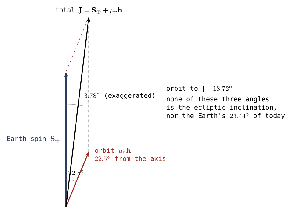
The fourth direction. The fourth direction named in the caption is the perpendicular to the ecliptic, set by the Earth’s motion round the Sun, independently of the internal parameters of the Earth–Moon pair. Part A establishes the starting inclination: 22.5° relative to the equator of the time of release, set by the latitude of the body’s centre. Part B defines the size and shape of the orbit the body enters at its release point, and Part C follows the orbital plane outward to the reference frame in which today’s 5.145° is measured.
Does the body enter an orbit that survives and recedes?
The corotation velocity is not necessarily identical to the circular orbital velocity appropriate to the release latitude. We compute the resulting orbital ellipse, and connect it to the tidal and survival tests developed in Paper 2.
Part A showed that a body released in corotation with the Earth at latitude enters an orbit inclined at the angle to the Earth’s equator. This part addresses the next question: what are the shape and size of this orbit, does the Earth’s tide then push it outward or draw it inward, and is the body far enough from the Earth to stay whole? The question carries real weight: an inclination has no meaning if the orbit that carries it spirals into the Earth or if the tide pulls the body apart.
Statement of the problem and the kinematic constraints. The first sentence of the box needs a word of explanation: the corotation speed given to a body at latitude is not the same as the circular orbital speed at the same radius. A body in corotation about the spin axis of the parent body does not move at the full distance from the centre of mass, but at the smaller local radius from the axis. As a result it moves more slowly than a body at the same distance over the equator, and at the equatorial corotation radius the speed of a body at an intermediate latitude is lower than the speed required for a circular orbit. The orbit it enters is therefore an ellipse, and the release location must be set so that this kinematic deviation is taken into account. This section finds where the orbit is a circle, and which orbit the Moon enters at its actual release point, a little beyond it.
B.1From release coordinates to an ellipse
An orbit around the Earth is in general an ellipse, and three numbers define its size and shape. The semi-major axis is half the longest diameter of the ellipse, the average of the nearest and the farthest distance; it sets the orbital period. The eccentricity measures how stretched the ellipse is: is a circle, and values approaching 1 describe a long, narrow ellipse. The nearest point of the orbit to the Earth is the perigee, at distance ; the farthest point is the apogee, at .
Analytic parametrisation of the orbital energy and speed. We define the dimensionless dynamical variables at the moment of release through the following coefficients:
where is the angular velocity of the Earth’s spin at the moment of release, the distance of the Moon’s centre of mass from the Earth’s centre, its geographic latitude, and the total gravitational parameter of the system ( the gravitational constant, and the masses of the Earth and the Moon). The parameter has a simple meaning: the body moves at the eastward speed , and is the ratio of the square of this speed to the square of the circular orbital speed at the same distance. Its threshold values define the character of the orbit: means an initial speed exactly equal to the speed of a circular orbit; means sub-orbital speed (the body is slower than required); , super-orbital speed (the body is faster than required); and would be the parabolic escape speed. represents the total orbital energy per unit mass; it is negative, so the body is gravitationally bound to the Earth, as long as .
Solving the orbit equations in the two-body approximation. For release conditions without a radial velocity component (the body moving at that instant neither towards the Earth nor away from it), when , and in the approximation of two point masses (the Earth and the Moon treated as point masses):
In words: the release distance and the single parameter fix the whole initial orbit. The farther lies from 1, the more eccentric the ellipse.
Positions of the apsides. For release takes place at apogee; for , at perigee; gives a circular orbit. The reason is direct: a body at sub-orbital speed for its distance begins to fall inward, so the release point is the farthest point of its orbit; a body at super-orbital speed swings outward, so the release point is the nearest.
Calibrating the local corotation line by latitude. At the radius — the equatorial corotation radius, where a body over the equator turning with the Earth has exactly the circular speed — a body at latitude is characterised by the parameter , which gives an initial eccentricity , not zero. The is the slowing explained above: the body circles the axis at , not at . A purely circular orbit, , is obtained only by moving the release distance to the latitude-corrected corotation radius, , where the speed carried by the rotation equals the orbital speed. This shift makes up the missing speed, because the speed carried by the spin grows linearly with radius while the circular orbital speed falls; equation (7a) gives the distance at which the two meet for a body at latitude .
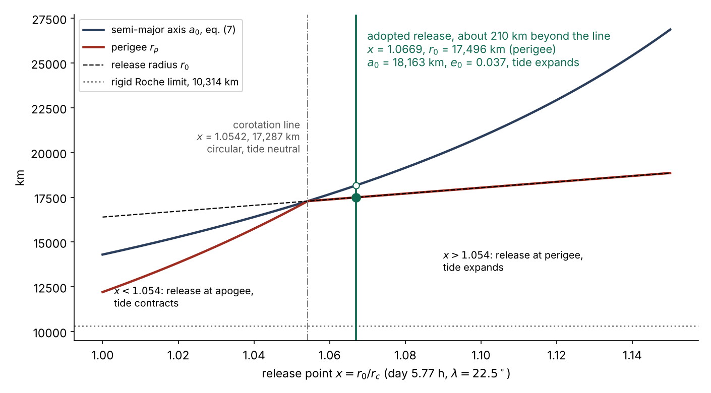
Numerical constraints of the detachment stage in the reference model. For an ancient day of 5.77 hours, the equatorial corotation radius stands at km (about 2.6 Earth radii), and at the release latitude the circular radius — the local corotation radius for this latitude — shifts to 17,287 km, about 900 km farther out, a dimensionless factor . The mechanical separation process begins when the Moon’s centre of mass reaches this line, and the final physical release takes place about 210 km beyond it, at km (), when a little more than half of the body’s mass (about 58%) has crossed the line. There , slightly above 1: the body is at a moderate super-orbital speed, so the release point is the perigee of the new orbit, and equation (7) gives a nearly circular orbit with , km and an apogee distance of 18,830 km. (An earlier version, with release about 100 km beyond the line, gave km, , km and an apogee of 18,005 km.) This release distance is the meeting point at which the reduced inclination and eccentricity tests of Paper 3, §C.5a, converge simultaneously.
B.2Combined results from Paper 2
Quantitative assessment of alternative release points. The table below applies equations (6)–(7) to five release points and adds two tests: the direction in which the Earth’s tide first moves the orbit, and the distance from the Roche limit. Here , the release distance normalised to units of the equatorial corotation radius. All rows are based on the release day of Paper 2, 5.77 hours (), and on . ( is the density ratio of core to mantle in the Paper 2 structure that gives this day.) The Roche column uses the rigid limit, because the body is rigid and round at the moment of release (Paper 2, §B.7).
| Earth day at release, h | , km | , km | , km | Initial terrestrial tidal contribution | Rigid Roche limit, 10,314 km | |||
|---|---|---|---|---|---|---|---|---|
| 2 | 1.00000 | 5.77 | 16,399 | 14,304 | 0.1464 | 12,209 | contraction | passes |
| 2 | 1.05420 | 5.77 | 17,287 | 17,287 | 0 | 17,287 | neutral | passes |
| 2 | 1.06695 | 5.77 | 17,496 | 18,163 | 0.0367 | 17,496 | expansion | passes |
| 2 | 1.08000 | 5.77 | 17,710 | 19,151 | 0.0752 | 17,710 | expansion | passes |
| 2 | 1.10000 | 5.77 | 18,038 | 20,880 | 0.1361 | 18,038 | expansion | passes |
Physical analysis of the table rows. The rows move the release point outward from top to bottom, and the tint shows the direction of the tide: blue for an orbit the tide draws inward, cream for the corotation line, where the tide is neutral, and red, deepening with distance, for orbits the tide pushes outward. In the first row (, on the equatorial corotation line) the local speed is lower than required, , and the release point is the apogee: the orbit dips to a perigee of 12,209 km, well inside the release distance. In the second row, on the corotation line for latitude 22.5, the tide is neutral, the eccentricity is zero and the three distances coincide at 17,287 km; the circular orbit is a single, well-defined point. The bold row is the adopted release, about 210 km beyond the line, where the tide widens the orbit from the first moment: the body is at a moderate super-orbital speed, the release point is the perigee ( km), and the orbit is nearly circular, , with km. In the last two rows the speed is higher still, and the orbit swings out to larger values of ; the eccentricity grows steadily on the far side of the circular point.
The origin of the release day. The release day of 5.77 hours is the result of two opposing processes acting on the initial 5.5-hour day: a slowing caused by the lengthening of the pear-shaped structure, and a simultaneous speeding-up resulting from the gathering of the core iron towards the parent body’s centre of mass (Paper 2, §A.4).
The direction of the tide. The Moon raises two tidal bulges on the Earth, one facing it and one on the far side, and the interaction is dictated by the ratio between the Earth’s spin rate and the Moon’s orbital rate. If the Earth turned exactly at the rate at which the Moon goes round it, the bulges would sit directly under the Moon, pull along the Earth–Moon line, and neither speed up nor slow down the orbit. When the spin rate is higher than the orbital rate, internal friction in the Earth carries the bulge slightly ahead of the Moon; the near bulge then pulls the Moon forward along its orbit, adds energy to the orbit, and the orbit widens — the Moon recedes, as it does today. When the orbital rate is higher than the spin rate, the bulge lags behind it, exerts a braking force, and the orbit shrinks, as happens today to Phobos, the inner moon of Mars. The test below decides which of the three cases applies at each release point.
The constant-time-lag test. The sign of the tidal orbital evolution in the table was computed in a constant time lag (Constant Time Lag) model, by averaging the power over the elliptical orbit; this is a defined test, not a rule independent of rheology. “Constant time lag” means that the bulge responds to the tidal pull after a short, fixed delay; “rheology” is the way the Earth’s material deforms and dissipates energy, and a full treatment will have to specify it. Appendix A gives the formula that reproduces the sign, in the framework of vector equilibrium tides [S4]. The formula, equation (14), compares two quantities: on the left, the Earth’s spin rate about the axis of the orbit, , divided by the mean orbital rate ; on the right, a function of the eccentricity alone, equal to 1 for a circular orbit. In the first row one obtains , so the terrestrial contribution to the evolution of is negative: the Moon on average outruns the turning Earth, and the orbit contracts. On the corotation line, , the two sides of the equation are equal: the orbit is synchronous and the tide is neutral. A body exactly on this line circles the Earth in the same time that the Earth turns beneath it, so its bulge stands directly beneath it and exerts no torque along the orbit. The Moon is released about 210 km beyond the line, at , and there the ratio is already : (an earlier version, with release about 100 km beyond the line, gave ), so the terrestrial contribution is positive from the first moment (row : ). The Earth turns faster than the Moon goes round, the bulge leads, and the Moon is pushed outward. Once the Moon begins to recede, its orbital rate falls further below the Earth’s spin rate, so the push continues: the neutral line is unstable in the outward direction, and the release state leads to sustained recession. Tides within the Moon may change the overall balance; the tide the Earth raises within the Moon is not included in this sign test (Appendix A).
The Roche limit. The Roche limit is the distance inside which the tidal pull of the Earth — the difference between its gravity on the near side and on the far side of the Moon — exceeds the Moon’s own gravity and can pull it apart. The test is made with the rigid limit, because the body is rigid and round at the moment of release (Paper 2, §B.7). Here is the Moon’s density; the denser the body, the closer it can approach without being torn. All five release points in the table lie outside the limit; the adopted release lies about 7,200 km beyond it (earlier versions, with release about 100 km beyond the line and with release on the line, gave 7,100 km and 7,000 km). Even the perigee of the first row, 12,209 km, lies outside the limit of destruction.
Why the rigid limit and not the fluid one. A specialist will ask why the rigid limit, and not the fluid one, is the right measure: for a fluid body that deforms freely under the tidal forces, with no shear resistance, the limit moves farther out (about 19,971 km for 2,600 kg m, Paper 2, §A.7.1), beyond the release radius. The answer lies in the mechanical state of the body. At the moment of release the Moon is round and its outer shell rigid, with an axis ratio of at most 1.04 (Paper 2, §B.7). The flattening and the later rounding of the lunar body took place earlier, in the stage of physical attachment (Paper 7, The Poles). A body with a rigid shell does not stretch along the tidal axis as a fluid drop does, and the rigid limit is the one that applies to it.
Figure 1 shows the same results as a continuous curve rather than four rows, so that the reader can see where the corotation line and the adopted release lie among all possible release points.
B.3 The release state
The separation mechanism and the kinematic threshold conditions. The Moon’s separation process begins when its centre of mass reaches the latitude-corrected corotation radius, 17,287 km. The final mechanical detachment takes place at 17,496 km, about 210 km beyond the synchronous line, when a little more than half of the body’s mass has crossed the line. The contact area exerts a weak mechanical resistance before detachment, and the body is pulled outward with force.
Properties of the first orbit. At this release distance the body’s speed is slightly higher than the speed required for a circular orbit: the point of detachment is the perigee of a nearly circular orbit (, apogee 18,830 km). Because the perigee lies beyond the synchronous line, the tide drives immediate recession, and the Moon recedes already from its first orbit. If the detachment forces had also given the body a small radial velocity component, the initial eccentricity would be somewhat larger, but with no shift of the angular-momentum vector and no change in the inclination (§A.2). The detachment itself is described in Paper 3.
Sensitivity of the final angle to the release distance. The distance beyond the corotation line dictates the shape of the first orbit and, through its size, the final angle. Moving the release outward raises the speed ratio , and with it and ; under the reduced law, the final angle grows as a weak function of . Paper 3, §C.5a, gives the full search; four of its rows at 22.5° show the trend:
| Offset beyond the line (km) | (km) | Final angle (reduced law) | |
|---|---|---|---|
| 0 | 0 | 17,287 | 5.020° |
| 100 | 0.017 | 17,696 | 5.079° |
| 210 (adopted) | 0.037 | 18,163 | 5.145° (observed) |
| 500 | 0.089 | 19,531 | 5.334° |
Table B.3. The initial orbit and the final angle of the reduced law as the release moves beyond the corotation line at 22.5° (Paper 3, §C.5a). The navy deepens with the final angle; green marks the adopted release, which returns the observed 5.145°.
Simultaneous convergence of the target measures. Release exactly on the corotation line would give a circular orbit, and the tide would carry it outward as a circular orbit, with no development of eccentricity. The present eccentricity therefore requires a release a little beyond the line. In Paper 3 the same offset, about 210 km beyond the synchronous line, also returns the Moon’s present eccentricity, 0.0549, for a young, hot body. This point is the meeting of constraints at which the two reduced tests, inclination and eccentricity, coincide; the full integration of Further work, item 1, carries the release state through the whole history. In this state the three basic conditions set out at the head of this part are met together: a nearly circular orbit, a positive outward tidal push, and a position well outside the mechanical limit of tearing.
The orbital starting point of the system is defined by the following parameters: km (18,163 km), , with the perigee at the release point, 17,496 km, and relative to the equator of that time. (Earlier versions, with release about 100 km beyond the line and with release on the line, gave km, , and km, , respectively.)
These values are the initial conditions for everything that follows: Part C follows the turning of the orbital plane as the orbit moves outward, and Part D examines how much of the 22.5° survives to the present distance.
How does the orbital plane change on the way out?
The initial inclination is defined against the plane of the parent body’s ancient equator, while today’s inclination is measured relative to the ecliptic. We identify the torques that turn the orbital plane, keeping the two reference planes fully separate.
Part B ended with an orbit inclined 22.5° to the Earth’s equator of that time. The observed 5.145° is measured relative to a different plane, the ecliptic — the plane of the Earth’s orbit round the Sun. This part explains why the reference plane changes as the Moon recedes, and what is required to follow the change. The point is essential: comparing an angle measured from one plane with an angle measured from another is comparing two different quantities.
C.1 Equator, ecliptic and the Laplace surface
Precession of the orbital plane and the twisting mechanisms. The orbital plane does not keep a fixed orientation in space. External perturbing forces twist it, and force the orbit’s axis to circle slowly around a central reference direction, like the axis of a tilted spinning top circling the vertical; this slow turning is called precession, and the inclination is measured from the plane about which it occurs. In the region close to the parent body, the Earth’s equatorial bulge produces a dominant twisting torque, which tends to pull the orbit towards the plane of the equator, and the orbit precesses about the plane of the equator. In the distant region, the gravitational perturbation of the Sun prevails, and the orbit precesses about the ecliptic, as the Moon’s orbit does today.
The Laplace surface and the scale of the transition. The Laplace surface defines the equilibrium orientations of the orbital plane under both influences together: at each distance it is the plane about which the orbit precesses. The surface coincides with the plane of the equator at short range, bends gradually, and converges to the ecliptic at long range. As the Moon recedes, the plane against which its inclination is effectively measured therefore turns from the equator to the ecliptic. The accepted scale for the transition, in the circular and quadrupole approximation, is [S5]:
where is the quadrupole moment of the gravity field, which measures the Earth’s equatorial bulge, is the Earth’s radius, the mean distance to the Sun and the Sun’s mass. The equation gives the distance at which the twisting effect of the Earth’s bulge and that of the Sun are about equal: inside the bulge dominates, and outside it the Sun. A larger bulge pushes the transition outward, but only weakly, through the fifth root.
Dependence on the internal structure. The transition equation shows what must be known: the gravitational moment , not only the rotation period. The relation between the two is dictated by the core, the shape and the cooling. A faster-spinning Earth bulges more, but how much more depends on the distribution of mass inside.
Order-of-magnitude estimate at release. An order-of-magnitude check only, with the present Earth radius and — that is, under the assumption that the bulge grows with the square of the spin rate, as rotational flattening does — gives about 17.07 Earth radii for the release day of 5.77 hours. The release radius, 17,496 km, is about 16.1% of this scale (earlier versions, with release about 100 km beyond the line and with release on the line, gave 16.0% and 15.9%), roughly one-sixth of the way to the centre of the transition (the release at of Part B, 17,710 km, would give about 16.3%). The Moon’s orbit therefore begins its outward journey deep inside the region where the equatorial bulge governs the plane, and its 22.5° is measured, at first, against the equator. The check supports a start in the region where oblateness is decisive; it does not replace a calculation of from the ancient structure, and does not determine how the transition radius evolved with time.
C.2 When can the adiabatic approximation be used?
A condition for adiabatic transfer. As the Moon recedes, the Laplace surface at its position tilts gradually from the equator towards the ecliptic. The question is whether the orbit follows the turning plane smoothly, keeping its inclination relative to it. A change is called “adiabatic” when it is slow enough for the orbit to complete many precession cycles while the guiding plane turns only a little; under these conditions the orbit tends to follow the plane, much as a top keeps circling a support that is tilted slowly.
Limits of the classical approximation. If the equilibrium surface changes slowly relative to the precession cycles, a conserved adiabatic action can be sought. This does not imply exact preservation of the inclination angle in every orbit of finite eccentricity and inclination. The classical Laplace surface is formulated for circular orbits, and the instability threshold of about 68.875° belongs to that defined framework [S5]. (This threshold is the tilt of the planet’s spin axis above which orbits lying on the classical Laplace surface become unstable in the transition zone.)
Constraints of the coupled system. A full solution requires combining the tilt of the Earth’s axis at that time, the line of nodes, the eccentricity, the recession rate and the evolution of the field. The line of nodes is the line along which the orbital plane crosses the reference plane; its orientation relative to the Sun decides in which direction the plane is twisted. The Earth’s tilt today is not a proven input for the past. The joint evolution of the Earth’s axis and the Moon’s orbit after release — the Earth–Moon axis system — is not solved in this series and is a subject for future work. The reduced calculation therefore does not fix a transition distance at 14.8 Earth radii, and does not establish an “exact transfer” of the equatorial angle to the angle relative to the ecliptic.
C.3The fossil figure and the Cassini state
Two further features of the present Moon record its passage outward. The fossil figure is the Moon’s present shape, which is more flattened than its present spin and distance would produce; it is read as a flattening frozen in at an early stage, when the Moon was closer and turned faster. A Cassini state is a configuration in which the Moon’s spin axis, the axis of its orbit and the axis of the plane about which the orbit precesses stay in one plane while they precess together; as the Moon receded it passed from one such state to another.
Complementary constraints. The Moon’s fossil figure and the transition between Cassini states are additional constraints, not evolutionary stages whose places on the path are derived directly from the release latitude. A coupled thermal-orbital model by Downey, Nimmo & Matsuyama found freezing of the figure before about 16 Earth radii under the conditions tested [S6]. Hence 21.6 Earth radii is not a unique freezing radius derived from observation, and the sequence “Laplace, figure freezing, Cassini” is not a general result.
The frequencies of the coupled system. An isolated comparison of two precession rates does not prove a new resonance in the range 17–19 Earth radii. Analysis of such a transition requires the frequencies of the full coupled system, including the solar perturbation and the mutual response of the two angular-momentum vectors. The paper does not claim that a channel for generating axial tilt is open only for the LEF path.
What we now have: the Moon starts with an inclination of 22.5° measured from the Earth’s equator, in the region where the equator governs the plane; the transfer of this inclination to the ecliptic, and the stages it passes on the way, are fixed by a full integration that includes the Earth’s bulge, the Sun and the axes of both bodies. Part D addresses how much inclination the tide removes on the way.
How much of the inclination survives, and in what time?
A match to a single angle is not enough if the calculation rests on a wrong initial orbit or reaches the present distance at the wrong time. We solve the reduced decay model exactly and test it against the thermal and orbital constraints.
The tidal forces that push the Moon outward act at the same time on the plane of its orbit, reducing its inclination as it recedes. This part takes the simplest law that describes this reduction, solves it exactly from the release state of Part B, and tests it against the second requirement every orbital history must meet: arriving at the present distance in the time available to it (the clock test).
D.1What the decay equation actually says
Consider the illustrative law, with measured from the equator of the parent body (the transition to the ecliptic is the subject of Part C):
In words: each small step outward, , reduces the inclination by a small amount. The minus sign dictates a fall of the inclination as the orbit widens; the factor gives equal weight to equal fractional steps in distance; and the factor sets the decay rate to zero for an orbit in the equator () and gives it a maximum at intermediate inclinations.
The additional damping coefficient. is an additional damping coefficient in the reduced model, and is not a solution for the lunar rheology. It stands for any extra loss of inclination, for example from dissipation of energy inside the Moon; means that only the basic tidal term acts. For a constant value, the exact integral is:
This is because . This is the tan-law: the tangent of the inclination falls as the inverse square root of the distance (for ). If the distance grows by a factor of four, the tangent of the inclination is halved. Replacing the tangent by the sine gives a different equation; it is an approximation valid only at small angles, where the two are nearly equal, and it shows a marked departure at a starting angle of 22.5°.
Numerical calibration of the final angle. To illustrate, insert , and (the present mean Earth–Moon distance). From the initial semi-major axis, about 18,200 km, to 384,400 km the distance grows by a factor of about 21, so falls by a factor of about 4.6. The table shows the sensitivity of the equation to a change in the inputs:
|
Insertion condition |
, km | Final angle in equation (11) | Conclusions |
|---|---|---|---|
| Release state (, about 210 km beyond the line, ) | 18,163 | 5.145° | Converges exactly to the observed value, 5.145°; the orbit begins in immediate recession (Part B) |
| Release 8% beyond the equatorial line | 19,151 | 5.282° | Low sensitivity to the release distance |
| Same release at | 18,163 | 5.788° | Sensitivity to the initial latitude |
The table changes one input at a time from the release state, and the deepening tint marks the growing departure of the final angle from the first row. The first row is the release state of Part B. The second uses the release at from the Part B table, 8% beyond the equatorial line, whose semi-major axis is 19,151 km: a semi-major axis about 5% larger than the adopted one shifts the final angle by only about one-seventh of a degree. The third keeps the release distance and raises the initial latitude to 25°, as a sensitivity case; the final angle rises by about two-thirds of a degree. (Earlier versions, with release about 100 km beyond the line at km and with release on the line at km, gave 5.079° and 5.713°, and 5.020° and 5.648°, for the first and third rows.) The final angle is thus dictated mainly by the release latitude, as equation (11) shows: it enters through , while the initial distance acts only through a square root.
Limits of the reduced model. All the rows examine the same reduced equation. The calculation is a solution of this equation alone: it does not integrate the evolution through the Laplace-plane transitions and the Cassini states, does not include the evolution of the eccentricity, and does not establish a prediction of the inclination relative to the ecliptic. In particular, the convergence of the final angle to 5.145° is a result of the reduced law for an orbit that begins in recession; it is not yet an integration through the transitions. The latitude at which the law returns 5.145° from the adopted release, km, is the series latitude itself, 22.5° (earlier versions gave 22.8° with release about 100 km beyond the line, 23.0° with release on the line, and before that a range of 23.3°–24.6°). Latitude and release distance trade against each other: a shift of half a degree in latitude moves the matching release distance by about 200 km (Paper 3, §C.5a). The agreement is therefore read together with the eccentricity test of Paper 3, and not from the angle alone.
Figure 2 draws the tan-law as a curve from the release state to the present distance.
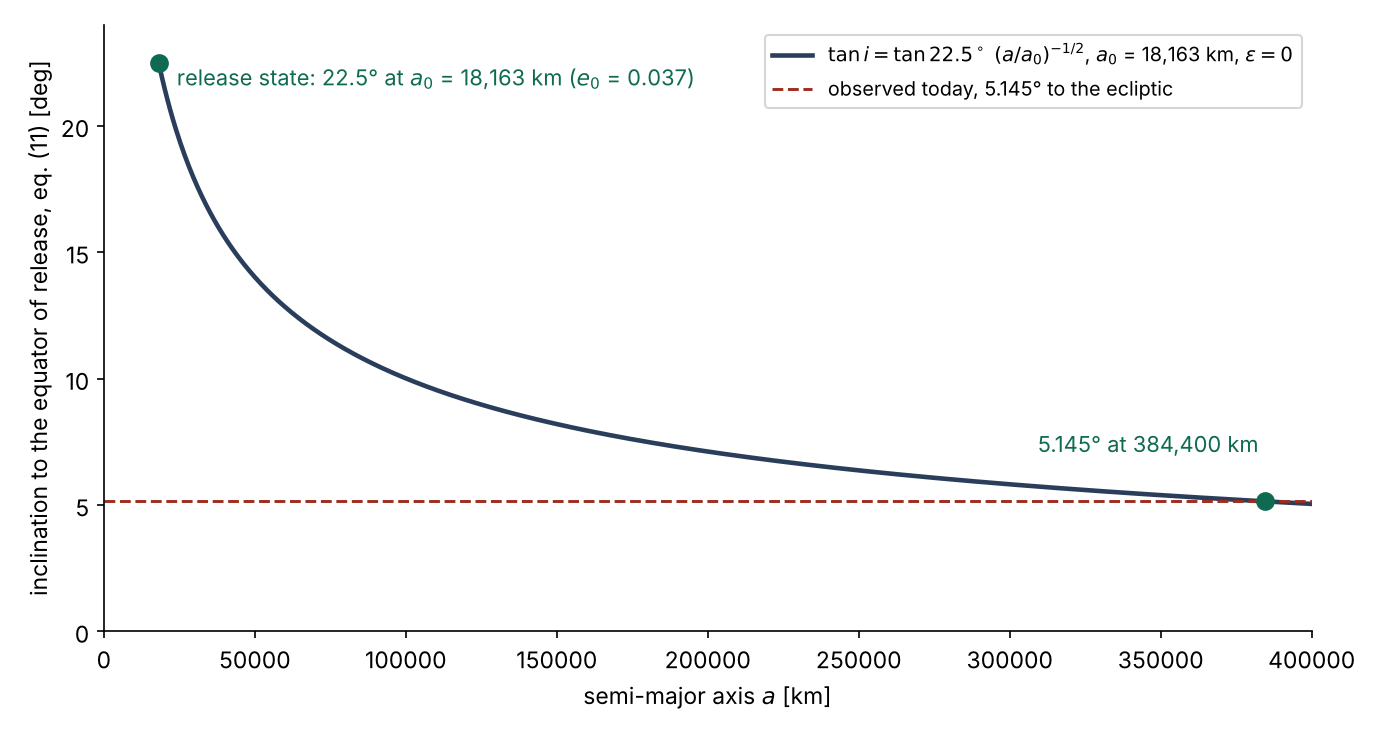
The curve shows a steep fall near the Earth, which flattens as the orbit widens. Most of the inclination is lost in the first stage of the journey, where each kilometre is a large fraction of the distance, while the late part of the journey, up to the present distance, affects the final angle only minimally.
D.2 Why cancelling does not solve the thermal history
The strength of the tide is usually defined by two coefficients. The Love number measures the deformation of a body under a tidal pull: 0 for a perfectly rigid body, and a higher value for a softer body. The tidal quality factor measures the dissipation of tidal energy to friction in each cycle: low represents strong friction, a bulge carried far from the line to the Moon, and fast orbital evolution; high represents weak friction and slow evolution. is the value for the Earth.
Cancellation in the division of the equations. The rate function that multiplies both and cancels completely in the division of the equations. This cancellation produces the explicit independence from within the illustrative law: equation (10) relates the inclination to the distance and not to time, so it gives the same final angle at any speed of recession. But if depends on the melting state at the time a given distance is reached, a change in the recession rate changes the melting state reached at that distance, and with it the damping coefficient. An everyday picture: the route of a car between two cities does not depend on its speed, unless the roads change with time; then the speed decides which roads are open when the car reaches them. In addition, the dissipation in the Moon need not be a constant multiple of the terrestrial tide.
Thermal-orbital constraints. Chen & Nimmo found in the models they tested that survival of the inclination places a strong limit, requiring in suitable scenarios [S7]. This is a model constraint, not a general material threshold for every material state. Solidification also does not switch off the tide: a solid body can dissipate energy. Models that include dissipation in the solid and in a magma ocean sharpen the conditions under which an ancient inclination survives [S6]. The thermal history of both bodies is therefore part of the inclination problem, and the cancellation of in the reduced law takes from it the ability to decide it.
D.3 One clock test suffices to expose the limit
The tan-law says nothing about time; the “clock test” completes it. The test requires that a simple tidal law, run outward from the release state, reproduce two boundary conditions: arriving at the present distance in a time that matches the age of the system, and obtaining the present recession rate. Both conditions must hold together.
For illustration only, we use a circular-equatorial law in the outward direction, with constant parameters:
In words: the recession rate falls very steeply with distance, as , because the tidal bulge weakens rapidly as the Moon recedes. The grouped constant gathers the tidal strength of the Earth, , the mass ratio of the Moon to the Earth and the size of the Earth; a larger means faster recession.
Integrating this equation gives:
This is the time to pass from the release distance to a final distance . Because of the high power , the term in is larger by orders of magnitude than the term in : nearly all the time is spent in the late, slow part of the journey, and the elapsed time hardly depends on the point from which the Moon started. It is, however, inversely proportional to , and therefore directly proportional to .
Numerical calibration. Inserting , , and gives a duration of about 1.60 billion years to the present distance, and a recession rate of about 3.70 cm/yr at that distance. The present rate is close to the observation, but the duration does not reproduce 4.5 billion years. Increasing to match the duration reduces the present rate by the same ratio: the time grows in proportion to and the present rate falls in proportion to , so no single constant value of can reproduce both measures.
Correcting the time horizon for the duration of construction. This is a calibration test of a simple law, not a history of the ancient Earth. The simple law is also not valid by itself in the inclined ellipse of Part B or near synchronism. Varying dissipation histories and oceanic resonances are the subject of detailed orbital models [S8]: the Earth’s oceans respond to the tide according to the geometry of their basins and the length of the day, and can pass through resonances in which the response is especially strong, so the present rate need not be the long-term average. If the construction lasted a substantial part of the ancient period, the time available after detachment must be computed from that date, rather than automatically adding 4.5 billion years after detachment. In the series, the construction stage lasts about 600 million years from the start of the bulge to release at 3.873 Ga, so the time available for recession after release is about 3.9 billion years, not 4.5. Against 3.87 billion years the clock fits at , and there the present rate falls to about 1.5 cm/yr; the conclusion is the same.
Figure 3 shows the clock test for every constant between 10 and 60.
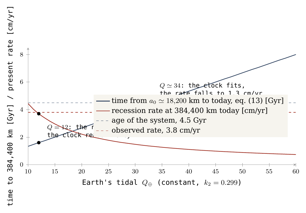
How to read Figure 3: the rising curve (navy line) represents the travel time, which grows linearly with ; the falling curve (red line) represents the present recession rate, which falls in inverse proportion to . Each solid curve has to meet its dashed target line, but the two meeting points lie at different values of — near 12 for the recession rate and near 34 for the age of the system. A history with a single constant cannot meet both points at once; it requires a dissipation that varies in time.
What we now have. The reduced tan-law carries the release latitude, 22.5°, to 5.145° at the present distance — the observed value — and the clock test shows that the time this takes is set by a dissipation that varied through the history. The full solution is a coupled thermal-orbital integration from the release state, and it is listed under Further work.
What has been proved and what will be tested?
A mathematical identity, a possible orbital branch and an observational reconstruction must be distinguished. The table defines for each claim its conditions, its quantitative result and its test, so that the assessment of the paper does not rest on a visual or verbal match.
Parts A–D took the Moon from the moment of release to the question of the present orbit. This part collects in one place what those parts establish, and how each result can be tested. The distinction in the box matters, because the three kinds of claim are tested in different ways. A mathematical identity, such as , holds wherever its inputs hold; the test is limited to verifying that it is applied in its proper place. An orbital branch, such as the release state of Part B, is one solution out of the space of solutions the equations allow; the test is to verify that the conditions it requires are met. An observational reconstruction, such as the present inclination, requires a full integration through the history of the system; the test is that a permitted history reproduces the observations.
The table below has one row for each claim. The columns are read in order: the claim; its basic assumptions; the number or sign it predicts; and the test protocol for the prediction. The tint of the rows follows the status of the claim, from top to bottom: navy for a geometric identity, cream for a result computed in this paper, and red for a result that requires the integration listed under Further work. The rows thus run from fixed identities to computed results, and from there to targets that require a full integration.
|
Claim |
Basic assumptions | Quantitative expectation | Test protocol |
|---|---|---|---|
| Source of the inclination — a geometric identity | Local release; eastward tangential velocity vector; latitude defined relative to the spin axis at the moment of release | Measurement of the centre-of-mass vectors at the end of the detachment stage; verification that there is no significant north–south velocity component and no torque turning the orbital plane | |
| The initial ellipse — two-body mechanics | An isolated two-body system; zero radial velocity, ; speed ratio in the range | Closed-form solution of equations (6)–(7) | Direct comparison with a short orbital integration; recomputation if velocity was added during detachment or in the field of an oblate Earth |
| Initial recession — computed (§B.2) | The release-state conditions and a tidal rheology model defined in advance | Averaging of the tidal power from both tidal systems, in the Earth and in the Moon | |
| Survival — Roche test passed (§B.2); deformation check open | Density, strength and thermal state consistent with the construction stage | The body survives the first perigee passages without breaking apart | Assessment of deformation, heating and mass loss under the conditions of construction (Papers 2 and 3) |
| The present inclination — requires integration | Joint evolution of the axis system, Laplace transitions, Cassini states and a dissipation function that varies in time | About 5.145° to the ecliptic, together with the present eccentricity | Full vector thermal-orbital integration (Further work) |
| Distance and clock — require integration | A detachment date and a time-dependent dissipation function consistent with each other | About 384,400 km and a recession rate of about 3.8 cm/yr today | Joint fit to the data and to the time constraints |
| The geographic link — requires an independent reconstruction | Reconstruction of the ancient latitude of the centre of mass | An independent latitude, including an uncertainty range | Structural and rotational reconstruction of the source site, not fitted to the orbit |
In plain words, each claim and its test:
Source of the inclination. The kinematic identity establishes that a body released while turning eastward with the Earth at latitude starts in an orbit inclined by to the equator of that time (§A.2). The test is the velocity of the centre of mass at the end of the detachment stage: the validity of the identity depends on this velocity carrying no significant north–south component, and on no torque during detachment turning the orbital plane. The identity is measured against the ancient equator, so it is not compared directly with today’s 5.145°, which is measured against the ecliptic (Part C).
The initial ellipse. The two-body orbit equations (6)–(7) define the size and shape of the first orbit from the release radius, the spin and the latitude (§B.1). Here means that the body has no velocity directly away from or towards the Earth at the moment of release, and is the range of the speed ratio for which the orbit is closed. The test is a short numerical integration of the same initial conditions, which should return the same perigee. Additional velocity components at the moment of detachment, or the field of an oblate Earth, require the ellipse to be rebuilt.
Initial recession. From the adopted release the Moon moves outward already from the first orbit: , where is the rate of change of the orbit’s size, and the brackets denote its average over one orbit. The test averages the tidal power from both bodies, the tide raised on the Earth and the tide raised on the Moon. At the adopted release this average is positive (§B.2).
Survival. The Moon survives its first perigee passages, close to the Earth. The adopted release lies about 7,200 km outside the rigid Roche limit of 10,314 km (§B.2), and the body is rigid and round at the moment of release (Paper 2, LEF Mechanism in Principle, §B.7). The remaining check is that the combination of density, strength and temperature that keeps the body whole through deformation, heating and mass loss is one that the construction of Paper 2 and Paper 3 (LEF Mechanism in Practice) produces.
The present inclination. The 22.5° of release becomes today’s 5.145° relative to the ecliptic. The reduced law of §D.1 already reproduces 5.145° at the present distance from the adopted release; the full test is a vector integration through the Laplace and Cassini transitions, with a time-dependent dissipation (Further work, item 1). The integration is to reproduce the present inclination and the present eccentricity together.
Distance and clock. The Moon reaches about 384,400 km in the time available to it since release, and recedes today at about 3.8 cm/yr. The clock test of §D.3 shows that a single constant value of the dissipation does not satisfy both conditions together; a simultaneous solution requires a dissipation history that varies in time. The test is a joint fit of distance, rate and time, which is to reach the present distance within the allowed age, with a dissipation history the Earth can have had.
The geographic link. The claim is that the release latitude can be traced to a place on the Earth’s surface. It is tested by an isolated structural and rotational reconstruction of the ancient latitude of the centre of mass, without fitting to the orbital parameters. The identity of the first row (equation (3) in §A.2) does not depend on this reconstruction, because it does not depend on where the site was.
The modern coordinate 25° north, 165° east, proposed in Paper 3, is not a direct measurement of the ancient release latitude. The paper adopts , the latitude of the centre of the contact area on the Moon, as the governing orbital parameter. The model distinguishes three locations in the pear-shaped structure (Paper 3). The base of the pear stood near Kiritimati, 1.9°N 157.5°W, roughly on the equator of that time. The back of the pear is defined by the coordinate 25°N 165°E. The release latitude, 22.5°, is the latitude of the centre of the contact area, about 3,000 km across, on which the Moon sat at the tip of the pear; this value is fixed throughout the paper. 25° is a sensitivity case only: the reduced law of §D.1 gives 5.788° from it, against 5.145° from 22.5°.
The width of the footprint of the contact area is not a degree of freedom for shifting the latitude of the centre of mass to fit the orbit, and the disappearance of a local gravitational perturbation is not proof that all dynamical information on the initial conditions has been erased. In other words, the size of the contact area does not allow the latitude to be moved within it until the orbit fits; the latitude is set by where the Moon’s centre of mass lay. Reconstructing a specific source site differs from constraining families of initial orbits: the first asks from which place on the Earth’s surface the Moon left; the second asks which release states lead to the present orbit. The second is an independent dynamical constraint, and it can be answered without the first.
Map of contribution and prior knowledge
The map separates the foundations of standard mechanics and the mechanisms known in the literature, which the paper takes as they are, from what the model adds. The table is read row by row: the first column names a component of the argument, and the second column states whether it is prior knowledge, an application of it, or the contribution of the model.
|
Component of the argument |
Status in the model |
|---|---|
| , Keplerian elements and conservation of angular momentum | Standard classical mechanics; the derivation is applied here explicitly |
| Change of orbital inclination by tides, resonances and encounters | Established physics and mechanisms studied in the literature [S2–S8] |
| Source of the initial inclination in release at non-zero latitude | Kinematic application; no claim of priority for the mathematical identity itself |
| Linking the release latitude to the release branches and the angular-momentum budget of Paper 2, and to the construction limits of Paper 3 | The original contribution of the model in this work; the starting orbit is fixed by the construction, with no free fitting |
| The full passage from the construction to the present Moon | The result of the series as a whole; the full coupled integration is listed under Further work |
The standard components. The first three rows rest entirely on accepted physics: the orbital angular momentum per unit mass (the cross product of position and velocity), the Keplerian elements that describe an orbit, and the known ways in which tides and gravitational encounters turn an orbital plane.
The contribution of the model. The fourth row defines what the model adds. The model does not choose the starting orbit to fit present data: the release latitude is tied to the release states and the angular-momentum budget computed in Paper 2, and to the limits of construction set in Paper 3; in this way the starting orbit is fixed by the construction rather than chosen to fit. The last row is the aim of the series as a whole.
Conclusions
The paper reaches six conclusions. The first three follow directly from the release state and are fixed in the model; the last three state what the reduced calculations show and what is required of the full integration.
A geometric source of the initial inclination. Local release at an eastward tangential velocity gives relative to the equator at the moment of release. This is a geometric source of the initial inclination in the LEF model. A body that leaves from a point off the equator, moving eastward with the Earth’s spin, moves in a plane that passes through the Earth’s centre and through the point of detachment; this plane is inclined to the equator at an angle equal to the latitude of that point.
The release radius and the corotation line. The same geometry fixes the release radius: off the equator, the corotation line, where the orbit would be circular, shifts outward and lies at ; at a 5.77-hour day and it stands at 17,287 km. The Moon’s separation begins when its centre of mass reaches this line, and release takes place about 210 km beyond it, at km, when a little more than half of the body has crossed the line; at this distance the reduced inclination and eccentricity tests of Paper 3 (§C.5a) meet. The corotation radius (16,399 km) is where a body on the equator, turning with the Earth, already moves at the speed of a circular orbit. Off the equator the body is closer to the spin axis and so moves more slowly; it reaches circular speed a little farther out, by the factor , equal to 1.0542 at 22.5°.
The initial orbit. Detached at this distance, the Moon enters a nearly circular orbit (, the release point is its perigee), the tide pushes it outward from the first moment, and it lies about 7,200 km outside the rigid Roche limit. The rigid Roche limit, 10,314 km, is the distance inside which the Earth’s tide would pull apart a rigid body of the Moon’s density.
The reduced tan-law. The solution of the reduced decay law is a law. The law exposes the sensitivity to the release conditions, and does not cancel the dependence of the full system on rheology and cooling. From the release state it gives 5.145° at the present distance, the observed value (§D.1). The agreement is the result of a single reduced equation, and the full vector integration is required to complete it.
The clock test. A tidal calculation with constant dissipation that approaches the present recession rate does not by itself reproduce the time elapsed since release. With the present rate comes out at about 3.70 cm/yr, but the present distance is reached within only about 1.60 billion years (§D.3); the dissipation in the Earth must have varied with time. A joint fit of four variables is required: distance, time, eccentricity and inclination.
A quantitative programme. The paper defines the passage from the construction stage to the orbital stage as a quantitative programme, in which all inputs are named. The full thermal-orbital reconstruction is the first item of Further work.
What we now have is an orbital starting point derived directly from the construction — km, , — and a list of the calculations and tests that lead from it to the present Earth–Moon system.
Formulas for reproducing the tidal test
This appendix gives the formula behind the column “Initial terrestrial tidal contribution” in the table of §B.2, and short code that reproduces the numbers of Parts B and D. The formula fixes the direction in which energy and angular momentum are transferred by the Earth’s tidal bulge, and answers a simple question: does the tide raised on the Earth push the Moon outward or draw it inward?
The sign criterion. In the constant time lag (Constant Time Lag) framework, the contribution of the parent body’s tide to is positive, and drives orbital recession, when [S4; application and calculation here]:
“Constant time lag” means that the response of the Earth’s tidal bulge to the Moon’s pull is delayed by a small, fixed interval; during this delay the spinning Earth carries the bulge forward, ahead of the Moon or behind it. The symbols are: the Earth’s spin rate; the inclination of the orbit to the equator, so that is the projection of the spin acting in the plane of the orbit; the mean motion, the Moon’s mean angular speed along its orbit, derived by Kepler’s third law from the semi-major axis and ; and the eccentricity. The left side therefore compares the angular speed of the Earth’s spin in the plane of the orbit with the Moon’s mean angular speed. In words: the Earth’s tide pushes the Moon outward when the Earth turns faster than the Moon goes round, by a margin dictated by the eccentricity on the right side.
For a circular orbit, , the right side equals 1 and the condition reduces to : the bulge runs ahead of the Moon and pulls it forward, as for a satellite beyond the corotation line. In an eccentric orbit the Moon moves faster than its average near perigee, where the distance is smallest and the tide strongest; the right side then exceeds 1, and the Earth must turn correspondingly faster for the net effect to be outward. The two eccentricity functions measure this:
Both equal 1 for a circle and grow with . Applied to the rows of §B.2, the test gives for release on the equatorial line (the orbit contracts), equality on the corotation line (the tide is neutral), at the adopted release , about 210 km beyond the line (the orbit expands from the first moment; an earlier version, with release about 100 km beyond the line at , gave ), and at (the orbit expands). On the corotation line the equality is exact by construction: the circular radius of equation (7a) is the radius at which .
Independent verification. The polynomials are not universal for every dissipation law. To separate mathematical verification from a material assumption, the sign of the tidal power was also computed by direct integration of the tangential and radial force components over a full orbital period, in the same model. The calculation does not include tides in the Moon, a solar torque or an active connection. The sign of the effect is thus confirmed independently of the series expansion; what remains an assumption is the constant-time-lag model itself.
Below is short Python code for reproducing the ellipses, the tidal sign and the inclination illustration from the coupled initial conditions of Paper 2. It is not presented as a 4.5-billion-year integrator.
from math import pi, sin, cos, tan, atan, sqrt, radians, degrees
G, M, m = 6.674e-11, 5.972e24, 7.35e22
K = G * (M + m)
lat = radians(22.5)
# r0 [km], Earth day at release [h]: coupled outputs of Paper 2
cases = [(16398.5, 5.77),   # on the equatorial line: release at apogee
         (17287.3, 5.77),   # corotation line: circular, tide neutral
         (17496.3, 5.77),   # adopted: about 210 km beyond the line
         (17710.4, 5.77)]   # 8
for r_km, day_h in cases:
    r = 1000 * r_km
    omega = 2*pi/(3600*day_h)
    B = omega**2*r**3*cos(lat)**2/K
    a, e = r/(2-B), abs(1-B)
    n = sqrt(K/a**3)
    f1 = 1 + 15.5*e**2 + 31.875*e**4 + 11.5625*e**6 + .390625*e**8
    f2 = 1 + 7.5*e**2 + 5.625*e**4 + .3125*e**6
    lhs = omega*cos(lat)/n
    rhs = f1/((1-e**2)**1.5*f2)
    toy_i = degrees(atan(tan(lat)*sqrt(a/384400e3)))
    print(a/1000, e, a*(1-e)/1000, lhs, rhs, toy_i)
The code applies the paper’s orbit equations and tidal test step by step, from the coupled initial conditions of Paper 2, for a release latitude of 22.5° and a 5.77-hour day at the moment of release. It examines four release radii: on the equatorial corotation line (16,398.5 km); on the corotation line for 22.5° (17,287.3 km; an earlier version gave 17,286.9 km, a value that leaves a residual ); at the adopted release, about 210 km beyond this line (17,496.3 km; an earlier version used 17,387.3 km, about 100 km beyond it); and at an offset of 8% beyond the equatorial line (17,710.4 km). For each case the code computes the speed parameter of equation (6), that is, the squared ratio of the speed carried by the rotation to the speed of a circular orbit at the same distance; then the semi-major axis and the eccentricity by equation (7); the mean motion ; the eccentricity functions of equation (15), written as decimals (15.5 is 31/2, 31.875 is 255/8, 11.5625 is 185/16, 0.390625 is 25/64, 7.5 is 15/2, 5.625 is 45/8, 0.3125 is 5/16); and the two sides of equation (14). The last line applies the reduced tan-law of equation (11) with from to the present distance, 384,400 km. Each output line gives in km, , the perigee in km, the two sides of the tidal test and the final angle. Running the code reproduces exactly the rows of §B.2 (14,304 km, 0.1464, 12,209 km; 17,287 km, 0, 17,287 km; 18,163 km, 0.0367, 17,496 km; 19,151 km, 0.0752, 17,710 km), the tidal test at the adopted release, and the angles 5.145° and 5.282° of §D.1.
Scope of verification and availability
This appendix defines what was checked, in what way, and what the checks do not cover, so that the reader can judge to what extent each number in the paper has been verified.
Numerical verification methodology. The original file was read in full, and the algebra of the decay equation was also checked against the original page. The structure and spin branches in the table were taken from the calculations of Paper 2, and their conversion to Keplerian orbital elements was rechecked. Within the check of Paper 2, an independent Newtonian integration of the reference orbit was carried out over a full orbital period, which reproduced the perigee radius and the return to the starting point, with a residual relative error in position of about . That is, after one full orbital period the integrated body returned to its starting point to within less than one part in a billion of its distance. This level of accuracy confirms that the orbit derived from equations (6)–(7) is the orbit that Newtonian gravity produces.
Limits of the check. The verification is limited to the monopole kinematics, in which the two bodies are treated as point masses. It confirms the orbital algebra, and does not test the reality of the connection or the validity of the rheology; the physical assumptions are those defined explicitly in Part E.
Sources and code. The names of the sources and their links were checked, and the claims attributed to them were limited to content accessible in the source pages and their abstracts; no equation-by-equation review of every cited paper is claimed. The document includes the code for the follow-on calculations. The complete structural solutions are included in the supplementary material of Paper 2; a full coupled thermal-orbital integration is not included, and is not reported as if performed.
Further work — openings for research
The calculations of this paper fix the starting point; the items below are the calculations that will carry it forward. Each item defines the fixed input that the present paper supplies, and the result the calculation is required to produce.
A coupled thermal-orbital integration from the release state. Fixed input: the initial conditions of the release state of Part B — release at km as perigee, km, , , a 5.77-hour day, and scaled to it as . Here measures the Earth’s equatorial bulge; for a fluid body the bulge grows with the square of the spin rate, hence the scaling. Required calculation: an integration through the Laplace-plane transition, through the Cassini state and with a time-dependent dissipation in both bodies, of the kind that existing secular integrators perform. The Laplace-plane transition is the distance at which the plane about which the orbit precesses changes from the plane of the Earth’s equator, which governs at short range, to the ecliptic, which governs at long range (§C.1). The Cassini state is the stable arrangement in which the Moon’s spin axis, the normal to its orbit and the normal to the ecliptic turn together (§C.3). A secular integrator follows the slow, orbit-averaged evolution of the orbit over billions of years. Result: the prediction of the present inclination.
The dissipation history of the Earth. Constraint: no constant fits both the present rate and the age (§D.3). measures how little of the tidal energy the Earth dissipates in each cycle: a low means strong dissipation and fast recession. Required calculation: ocean-resonance models of the early Earth, initialised from the 5.77-hour day at the moment of release (rather than from the 6.4-hour day of the earlier stage, of the pear alone). An ocean-basin resonance occurs when the natural sloshing period of the basin approaches the tidal period; the dissipation then rises sharply, and it changes as the day lengthens and the continents move [S8]. Result: the rate function the integration requires.
The Earth–Moon axis system. The angle of about between the Earth’s spin vector and the total angular-momentum vector at the moment of release (§A.3) belongs to the Earth–Moon axis system, future work outside the bounds of the series, and no claim is made here about it.
The magma-ocean switch. Constraint: the survival of the inclination depends on whether the lunar magma ocean had solidified before the Moon reached 20 Earth radii; the constraints on this from the models of [S6] and [S7] are discussed in §D.2. The magma ocean is the molten outer layer of the young Moon; while it is liquid, the Moon dissipates tidal energy strongly, and the inclination is damped faster. Required calculation: an asymmetric thermal model of a Moon with a one-sided lid — thick on the far side and thin on the near side, where the maria were still hot at the time of detachment (Paper 3). A lid of uneven thickness cools at a different rate from the uniform shell that the published models assume. Result: the solidification time, that is, the moment at which the switch acts, for this body and not for a symmetric one.
The fossil figure. Constraint: a body that went through outward rounding, flattening and inward rounding while it sat as a squashed ball on the tip of the pear carries its figure from that stage, not from a later tidal lock. In the LEF model the flattening and rounding of the lunar body took place while it was still attached (Paper 7, The Poles). The fossil figure is the slight departure of the Moon’s shape from a sphere that its rigid outer shell has preserved from an earlier time; the degree-2 shape is the largest-scale part of that departure, its overall elongation and flattening, as measured in the gravity field. Required calculation: derivation of the relation between the geometry of the squashed ball on the tip of the pear (Paper 3) and the present degree-2 shape, a calculation not yet made. Result: a test of whether the shape left by the attached stage matches the present one.
Code availability
The reproduction package. All numerical results of the paper are fully reproduced by the scripts of the LEF reproduction package (Python 3, numpy, scipy), which prints the values of each section from the inputs stated in the text.
Archiving and access. The package is attached to this preprint as supplementary material (LEF_code_and_data.zip). An earlier version of the series and of the package is deposited at doi:10.5281/zenodo.22743615.
References
[1] Duran, Z. (2026). The Model. LEF, Paper 1.
[2] Duran, Z. (2026). LEF Mechanism in Principle — Corotation and Angular Momentum. LEF, Paper 2. Integrated working manuscript, including the release-latitude and orbital-survival calculations.
[3] Duran, Z. (2026). LEF Mechanism in Practice — Pressure and the Pear. LEF, Paper 3. Integrated working manuscript; the connection and the release margin beyond corotation.
[S1] Williams, D. R. (2024). Moon Fact Sheet. NASA Goddard Space Flight Center, NSSDCA. https://nssdc.gsfc.nasa.gov/planetary/factsheet/moonfact.html.
[S2] Pahlevan, K., & Morbidelli, A. (2015). Collisionless encounters and the origin of the lunar inclination. Nature, 527, 492–494. Authors’ copy: arXiv:1603.06515.
[S3] Ćuk, M., Lock, S. J., Stewart, S. T., & Hamilton, D. P. (2021). Tidal Evolution of the Earth-Moon System with a High Initial Obliquity. Authors’ copy: arXiv:2107.03353.
[S4] Correia, A. C. M., Laskar, J., Farago, F., & Boué, G. (2011). Tidal evolution of hierarchical and inclined systems. Celestial Mechanics and Dynamical Astronomy. DOI: 10.1007/s10569-011-9368-9. Authors’ copy: arXiv:1107.0736.
[S5] Tremaine, S., Touma, J., & Namouni, F. (2009). Satellite dynamics on the Laplace surface. The Astronomical Journal, 137, 3706–3717. Authors’ copy: arXiv:0809.0237.
[S6] Downey, B. G., Nimmo, F., & Matsuyama, I. (2023). The thermal-orbital evolution of the Earth-Moon system with a subsurface magma ocean and fossil figure. Icarus, 389, 115257. Authors’ copy: arXiv:2209.00935.
[S7] Chen, E. M. A., & Nimmo, F. (2016). Tidal dissipation in the lunar magma ocean and its effect on the early evolution of the Earth–Moon system. Icarus, 275, 132–142.
[S8] Farhat, M., Auclair-Desrotour, P., Boué, G., & Laskar, J. (2022). The resonant tidal evolution of the Earth-Moon distance. Astronomy & Astrophysics, 665, L1.
Use of AI tools: The author used AI assistants (Claude, Anthropic; ChatGPT, OpenAI; Google’s AI search assistant) to write and run the computation scripts, to analyse the catalogues and maps, to prepare figures and tables, to discuss the scenarios, and for language editing and translation. The model and its conclusions are the author’s. The author checked the content and takes full responsibility for it.