LEF Mechanism in Principle
Corotation and angular momentum
The computational environment table
The calculations of this paper describe an early terrestrial parent body — the young Earth before the Moon left it — in the LEF scenario. Because the system changes during the process (mass moves from one body to the other, the shape and the spin change), every number below belongs to a defined state: the state before the division of mass, a computational reference state used for comparison, or the coupled final state at release. Keeping these states apart prevents a value from one moment being used at another. Appendix G contains the full environment, E01–E70; the table here lists only the quantities needed for Paper 2.
The table has three columns. The first names the quantity, the second gives its value or definition, and the third says what kind of number it is: an assumption of the system, an input chosen for the model, a value computed in this paper, or a value used only to test how sensitive the result is. The reader can use the third column to see at once which numbers are put in and which come out.
|
Quantity |
Value or definition | Status |
|---|---|---|
| Parent mass at the start of the account | 6.0455×1024 kg — Earth and Moon together | System assumption, no mass loss |
| Parent mass after the transfer | 5.972×1024 kg | Model input |
| Transferred mass | 7.35×10²² kg | Model input |
| Initial rotation period | 5.5 hours | Adopted reference value |
| Initial volumetric radius | 6,517 km | Input; includes an adopted expansion of 120 km |
| Initial equatorial radius | about 6,721 km | Computed in the Maclaurin model |
| Initial mean density | about 5,214 kg/m³ | Derived from mass and volume |
| Initial structure for the budget | homogeneous, approximately | Reference assumption, not a conclusion from incomplete differentiation |
| Final structure in the sensitivity test | two layers; –, – | Computed scenarios |
| Corotation in the original reference | 15,818 km at 5.5 hours, with GM of the final Earth mass in the test-particle approximation | Computational definition; not an insertion of the full initial mass |
| Earth day and corotation line at release | 5.77 hours; 16,331 km (16,399 km two-body), core centralising, | §A.4, §B.1 |
| Release off the equator | 25° relative to the spin axis at the moment of release | Sensitivity-test assumption, not a measured ancient latitude; the adopted release latitude is 22.5° (Paper 4) |
| Body density in the Roche test | 2,600 kg/m³ | Input; 1,500 and 3,340 tested as sensitivity |
| Temperature, volatiles and viscosity | vary between regions; no approved numerical profile | Not replaced by modern values |
| Gravity | depends on mass, distance and shape in every state | No single gravity figure for the whole process |
| Duration of construction | not computed in Paper 2 | The 600 Myr window is kept in the working scenario, not as a measured time |
A few rows need a word of explanation. The parent mass at the start, 6.0455×1024 kg, is simply today’s Earth and Moon added together: nothing is assumed to escape, so the whole Moon was once part of the Earth. The initial radius, 6,517 km, is larger than the Earth’s today because a young, hot Earth is expanded; the adopted expansion is 120 km. A spinning fluid body bulges at its equator, and the Maclaurin model — the classical equilibrium shape of a uniformly dense, spinning fluid body, a flattened sphere — turns that volume into an equatorial radius of about 6,721 km. The test-particle approximation treats the released body as a small particle in the field of the central mass, so that only the Earth’s mass enters the formula; the coupled two-body value (16,399 km instead of 16,331 km) shows how small this simplification is. The two-layer rows use , the ratio of the radius of the dense inner layer to the radius of the whole body, and , the ratio of the inner density to the outer density; is a uniform body and larger means more iron gathered towards the centre. The 25° row is a sensitivity test, used to see how much the result changes when the release does not lie on the equator; it is not the adopted value, which is 22.5° (Paper 4). Where the table says that a quantity has no single value — temperature, viscosity, gravity — the paper does not borrow a modern value in its place. The 600 Myr construction window is the working scenario of the series: roughly 400 Myr for the bulge and the pear, about 100 Myr of flattening and about 100 Myr to release at 3.873 Ga. Paper 2 does not compute this duration and does not depend on it.
Before a lunar reservoir separates, the mass of the lunar material is included in the parent body. After the transfer the same mass is assigned to the second body. The distinction between the total initial mass and the mass used in the reference calculation prevents double counting and the mixing of states.
In practice this means: the 7.35×10²² kg of the Moon is counted once. Before the transfer it is inside the Earth’s 6.0455×1024 kg; after it, it is the Moon, and the Earth keeps 5.972×1024 kg.
The idea. Anything that is part of a spinning planet, or still attached to it, turns with it: it goes round once in every planetary day. This is corotation. The farther from the centre such material is, the faster it moves, because its speed is the spin rate times the distance. The speed needed for a free circular orbit does the opposite: it falls with distance. At one distance the two speeds are equal — the corotation radius. Material carried out to that distance while still turning with the parent, and released there, already moves at orbital speed; nothing has to throw it.
The question. The paper examines whether transferring lunar material outward from a terrestrial parent, while corotation is maintained, can lead to a state whose orbital velocity and angular-momentum budget approximately match the present Earth–Moon system. (Angular momentum is the amount of rotation a system holds; internal processes can only pass it from one part to another, and only outside forces such as the Sun’s tides can remove it.) The central distinction is between the required velocity at release and the mechanical capacity and angular-momentum budget needed to reach that state. In a central-field model the corotation radius follows from equating the rotational speed and the orbital speed. For an initial period of 5.5 hours the reference values are 15,818 km and 5,020 m/s.
The budget. The parent is described as a uniform Maclaurin spheroid (the flattened equilibrium shape of a spinning fluid body) with a volume-equivalent radius of 6,517 km. The computed initial angular momentum is about , about 0.7% above the sum of the magnitudes of the present angular-momentum components — a small surplus, which is what the later loss to solar tides requires. Vector addition at the angles tested gives a surplus of about 1.5–2.5%; this is a sensitivity test, not a full vector reconstruction of the evolution. The surplus depends on the nearly uniform structure and on the adopted expansion.
The release. Two processes change the Earth’s spin during the transfer: the lengthening pear carries rotation outward and slows the Earth, and the centralising core — iron sinking inward — speeds it up. They act together; with the Earth day at release is 5.77 hours and the corotation line lies at about 16,400 km, where the Moon’s centre of mass is released. The angular momentum added to the material is about 15.6% in the base calculation and about 16.5% in the coupled solution; the final orbital angular momentum is about 17.7% of the initial budget in the coupled solution with the pear alone (), and about 17.0% in the release state with (§B.1). These are transfers within the system.
The result. The paper establishes the kinematic solution and the budgetary end state of the route: the speed a corotating mass needs is supplied by the rotation itself at the corotation radius, and the angular momentum the transfer requires is available in the parent. What the route then requires of the mechanism — that the body be released beyond corotation, that it survive the years it spends inside the fluid Roche limit, and that the connection carry the load until then — is stated as a set of explicit conditions in Part D. Paper 3 examines those conditions.
The layout. Part A states the problems the route must meet; Part B solves them in the same order; Part C summarises; Part D lists claims, tests and requirements; Part E concludes. Appendices A–G hold the derivations and the full environment.
The Moon’s material left the Earth while still turning with it, and was released where the speed it already had was the speed a free orbit requires. That place is the corotation radius: 15,818 km for a 5.5-hour parent, 5,020 m/s. The objection that closed the fission route — an angular-momentum budget four times too large — was evaluated at the parent’s surface, under a release condition this route never uses. Evaluated at the corotation radius, the parent’s budget exceeds the present system’s by about 1%, with the sign that solar tidal loss requires, and the classical route needs 2.74 times what this one needs.
The route is specific about what it needs. A parent still at an early stage of sorting at the start of the transfer (), thermally expanded by 98–520 km; a body released beyond, not at, the corotation radius; an interior stiff enough to survive – years inside the fluid Roche limit; and a connection able to carry the load until then. Each is a definite requirement, each is passed to the paper that supplies it, and each is listed in §D.3. The requirements of the model, and what would test it, are collected in Paper 11 (The Requirements).
Why the old objection does not apply. Classical fission asked the Earth to throw material off its own surface. At the surface of a 5.5-hour parent the rotation gives about 2,133 m/s, while a free orbit there needs about 7,701 m/s (§A.1.2). The only way to close that gap at the surface is to spin the whole Earth much faster, and a faster spin means more angular momentum: at the classical point where a spinning fluid body becomes unstable (the Jacobi bifurcation, §A.6.5) the parent needs 2.74 times the angular momentum the Earth–Moon system has today, and the older reference calculation, made at another point of the same sequence, gave about four times. The system does not have that much, and this is why fission was abandoned. The LEF route closes the gap in a different way: not by spinning faster, but by carrying the material outward while it turns with the Earth. Its speed grows with distance at the same spin rate, until at the corotation radius it equals the orbital speed. The spin the Earth needs for this is the spin it would have had if all of today’s angular momentum were returned to it — about 5.5 hours (§A.2) — and the budget then needed is 1.007 times today’s. An everyday picture: a child on a roundabout who walks from the centre to the rim moves faster at the rim without anyone pushing the roundabout harder.
What the requirements mean. is the moment-of-inertia coefficient: it measures how the mass of a body is spread between centre and surface. A uniform sphere has ; today’s Earth, with its iron core, has about 0.33. The route needs at the start of the transfer, that is, a parent still at an early stage of sorting: an Earth whose mass is less concentrated toward the centre stores more rotation at the same spin. The organisation of the Earth’s core is one continuous process that never stopped. During the bulge it was at its beginning; while the pear grew it continued; and after release it went on while the Earth took the pear back in. There was probably never a fully uniform period: the earlier the stage, the less sorted the Earth. Iron may already have been gathering in the core at the start; the process continued. The young Earth must also be hot and therefore larger than today: an expansion between 98 and 520 km is admissible, and 120 km is adopted. The body must be released beyond the corotation radius and not exactly on it: exactly on the line the tide is neutral and gives no push either way, while a body lying even slightly beyond the line is pushed outward by the tide, so that it recedes from the start (Paper 4); the margin needed is small, , about 210 km (Paper 3, §C.5a). The fluid Roche limit is the distance inside which the Earth’s tide would pull apart a body held together by its own gravity alone. A body with internal strength survives closer in, down to its rigid limit; the Moon at release is rigid and round, with its flattening and rounding completed earlier, while it was still attached (Paper 7). The connection between the two bodies — the pear — must carry the load until release. These requirements are not hidden in the results; they are collected in §D.3, and Paper 3 tests them.
Introduction — Part A: the release condition in the context of existing models
Two kinds of evidence bear on the Moon’s origin: how its material could have reached orbit (the dynamics of separation) and whether its composition matches the body it came from. Darwin’s work on tides and rotation is part of the historical background for examining the evolution of the Earth–Moon system [6]; his fission idea — that a fast-spinning Earth shed the Moon — is the classical form of a terrestrial origin. In this paper the quantitative comparison with classical fission is made through a defined equilibrium configuration; a result for one configuration must not be converted into a bound on every possible path. In other words, showing that one particular fission path needs too much angular momentum does not show that every path from the Earth does.
In the giant-impact family of models, the Moon forms from debris after another body strikes the Earth, and the isotopic composition places constraints on the mixing of terrestrial and impactor material. Different versions of the model exist, and the constraints depend on the compositions and on the manner of mixing [7]. In the LEF scenario, construction from a shared terrestrial reservoir is examined: the Moon is made of the Earth’s own material, so a close isotopic match follows directly. A shared source provides a basis for compositional comparison, but does not replace the test of transfer to orbit. That test is the subject of this paper.
The focused question of this paper is whether carrying mass outward in shared rotation changes the velocity condition and the angular-momentum budget relative to direct release from the surface. The answer the paper gives is that it does: the release condition is moved from the surface to the corotation radius, and both the speed and the budget then fit. The mechanism of construction — the feed from within and the rise of the outer shell as the surface of the same body — is the subject of Paper 3, LEF Mechanism in Practice. The present paper defines the physical conditions it must meet. The division is deliberate: Paper 2 asks whether the route is possible in principle, using standard physics; Paper 3 shows how it is carried out.
Introduction — Part B: what the paper presents
The paper is built as a set of problems followed by their solutions, so that each objection is met in the place where it is raised. Part A sets out the problems the route must meet, one by one: the velocity gap that led to the rejection of classical fission, what must be calculated, the pear that connects the Earth to the corotation line, the offset between the lengthening pear and the centralising core, corotation itself, the angular-momentum budget, the Roche limit and the direction of tidal evolution. Part B solves them in the same order, starting from one calculation. Part C summarises what has been shown; Part D collects the claims, tests and requirements; Part E states the conclusions. Appendices A–G give the derivations, the sensitivity scans, the Roche calculations and the full computational environment, so that every number in the main text can be traced and reproduced.
To keep the principle clear, the calculation and the whole of this paper treat the release of the Moon from the equatorial plane. Paper 4 shows that the Moon left from another latitude — 22.5, the centre of the contact area — and recomputes the release there.
The equatorial plane is the simplest case: there the spin carries material fastest and the corotation radius is a single distance. Release from a higher latitude changes the numbers somewhat but not the principle; the size of the change is shown by the 25° sensitivity test of the environment table, and the adopted case of 22.5° is computed in Paper 4.
The problems before us
Each section of this Part states one condition that a body built from the Earth’s own material must meet if it is to reach orbit whole. Part B answers them in the same order.
This Part sets out the physics the route has to satisfy, one problem at a time. It begins with the difficulty that closed the classical fission route — a body leaving the surface of a fast-spinning Earth does not have the speed of an orbit — and then asks, in turn, where that speed is reached, what connects the Earth to that place, how the Earth’s spin changes while the material moves out, whether the angular momentum suffices, whether the body survives the Earth’s tide, and in which direction it moves afterwards. Each section ends with a defined quantity that Part B then computes.
A.1The problem: the velocity gap
A.1.1Two separate dynamical questions
A terrestrial-origin scenario requires an explanation for the transfer of material from the parent body to a free orbit. A compositional match can support a shared source without determining how material reached orbit: two bodies may be made of the same material and still leave open the question of how one of them came to circle the other. The focus of this paper is therefore the dynamics. The original historical review is examined here by comparing defined equilibrium configurations, and not by asserting that every terrestrial-origin path is subject to the same fission threshold.
Two questions have to be kept apart. The first question is under what conditions the velocity of the material is consistent with a free orbit — that is, whether, at the moment it is let go, the material moves fast enough sideways to keep falling around the Earth without falling back onto it. The second question is whether the angular momentum available at the start of the process permits the end state and the later evolution. Changing the release condition can change the velocity test, but the overall angular-momentum balance must still be satisfied. A route can pass the first test and fail the second, so both are computed.
Angular momentum and the moment of inertia. Angular momentum is the quantity of rotational motion a body carries. For a spinning body it is the product of how fast it turns and how its mass is spread around the axis. The spin angular momentum is:
Here is the angular velocity (the angle turned per second, divided by the period) and is the moment of inertia: the sum, over every piece of the body, of its mass times the square of its distance from the spin axis. The moment of inertia measures how far from the axis the mass sits; mass far from the axis counts much more than mass near it, because the distance enters squared. For a body of mass and equatorial radius it is convenient to write , where the dimensionless coefficient records how the mass is distributed: a uniform body has , and a body with a dense core has a smaller .
Angular momentum is conserved: in a system on which nothing outside exerts a twisting force (a torque), its total cannot change; it can only be passed from one part of the system to another. For the Earth–Moon system the only significant outside torque is the tide raised by the Sun, which removes about 1% over the system’s history (§A.2). This conservation is what makes the problem calculable: whatever the Moon carries in its orbit today must once have been in the spin of the parent.
Transferring material outward in corotation — that is, while it keeps turning with the parent at the parent’s own angular velocity — requires the parent to supply additional angular momentum to that material, because the same angular velocity at a larger distance means a larger moment of inertia for that material. In the absence of an external torque, this is a redistribution of existing angular momentum: what the material gains, the parent’s spin loses.
A.1.2Release from the surface
We first examine the classical case: material let go directly from the equator of a fast-spinning parent. In the reference state the period is hours and the equatorial radius is km. Therefore, since 5.5 hours are 19,800 seconds:
Two speeds must now be compared at the equator. The first is the speed the rotation itself gives to a point on the surface, : the angular velocity times the distance from the axis. The second is the circular orbital speed : the speed at which a free body at that distance would keep falling around the Earth in a circle, its centrifugal tendency exactly balancing gravity.
Even with a day of only 5.5 hours, the surface moves at less than a third of the speed an orbit there requires. The velocity difference, in the rounding of the original reference calculation of this paper, is about 5,568 m/s. This is the velocity gap.
What orbit would such material follow if it were simply let go? Without an additional radial velocity, the specific energy (the orbital energy per kilogram, kinetic minus gravitational) and the semi-major axis (half the long axis of the resulting ellipse) are:
The energy is strongly negative — the material is deeply bound — and the semi-major axis, 3,495 km, is about half the parent’s equatorial radius. The release point is the farthest point of this ellipse, so the whole of the rest of the path lies deep inside the parent. Under these initial conditions the Keplerian orbit penetrates the parent body: the material simply falls back. Surface velocity alone therefore does not provide a free orbit that remains outside it. This is the core of the classical objection to fission: to close the gap at the surface the parent would have to spin several times faster, which requires far more angular momentum than the Earth–Moon system holds (§A.6.5).
The numbers in §A.2 preserve the original reference comparison, in which GM of the final Earth mass was used. They are not a calculation of the exact field of the whole initial parent. This definition distinguishes the reproduced reference comparison from the overall budget in §A.6.
A.1.3The transfer condition examined
The LEF route does not let the material go at the surface. In the scenario examined, the material rises while still attached and receives angular momentum, so that it keeps turning with the parent as it moves out. The two speeds then behave in opposite ways. The velocity grows with distance, because a point that turns once per day travels a larger circle the farther out it is — as a child walking outward on a turning roundabout is carried round faster and faster. The orbital speed decreases, because gravity weakens with distance and less sideways speed is needed to balance it. The gap of §A.1.2 therefore narrows as the material rises, and at one distance it closes.
The paper computes the point of equality and the angular-momentum cost of the transfer; the ascent process itself is a separate mechanical question. Paper 3, LEF Mechanism in Practice, examines the transport capacity and the connection; the detailed pressure calculation is outside the budget calculation presented here. The orbital initial conditions are handed to Paper 4, The Orbit.
A.2What must be calculated
The problem now has a definite shape. Five quantities must be calculated: where the Moon is released, with what Earth day, whether the angular momentum suffices, whether the body survives the tide, and whether it recedes afterwards.
Why 5.5 hours. The starting spin is not chosen freely; it follows from conservation of angular momentum run backwards. All of today’s Earth–Moon angular momentum, kg m s — the Earth’s spin together with the Moon’s orbit — is returned to the spin of a young, hot, expanded Earth still at an early stage of sorting ( as the calculation input). “Expanded” means that the hot early Earth was somewhat larger than the cold Earth of today; “an early stage of sorting” means that the organisation of the core had only begun, so the mass was spread nearly uniformly and the uniform value describes it closely. Putting the whole budget into the spin of such a body gives the period: In words: a body with moment of inertia carrying angular momentum turns at , and its period is . Solar tides have since removed about 1% of the system’s angular momentum (about 1.35% when the receding Moon is followed; Eulenfeld & Heubeck 2023; Canup 2004). A period of 5.5 h therefore carries today’s angular momentum and the roughly 1% that was lost: it is slightly shorter than 5.54 h because the early system held slightly more. A young Sun more massive by a few per cent raises this loss only to 1–2%.
A.2.1The reference state
For and hours, the distance at which the speed of rotation equals the orbital speed — the corotation radius, derived in §A.5 — and the common speed there are:
This is the central number of the paper. At 15,818 km, more than twice the parent’s equatorial radius, a body that turns once every 5.5 hours with the Earth already moves at 5,020 m/s, which is exactly the speed of a circular orbit at that distance. A body held there in corotation and then let go does not need any additional push: it is already in orbit.
The distance is measured from the centre of the central body in the test-particle approximation, in which the orbiting body’s own mass is neglected in the gravitational pull. Substituting this radius into the two velocity formulas confirms that the speeds are equal.
The derivation is an application of the equations of motion in a central field [8]. If an initial state is computed with the full parent mass, must be inserted in the formula. The value 15,818 km remains the reference defined in the table; the coupled solution in §A.4 explicitly includes the division of mass.
A.3The pear
The corotation radius lies far above the surface, so something must carry the material there while it keeps turning with the Earth. In the model this is the pear. The connection is a hill that rises from the Earth: a base about 9,000 km wide at the surface, sides that form a single arc without a waist, and a contact disc 3,000 km wide at the Moon. It bridges about 7,800 km between the Earth’s surface and the Moon and lies entirely inside the corotation line, so it is pulled inward: everywhere along the pear, gravity is stronger than what the rotation needs to keep the material circling, so the pear’s own material is held by the Earth and does not fly off. Only the body at its tip reaches the line. Its length and mass are a requirement: the Moon was released whole, so a pear must exist that meets the conditions. How the pear is built and how it carries the load are the subject of Paper 3.
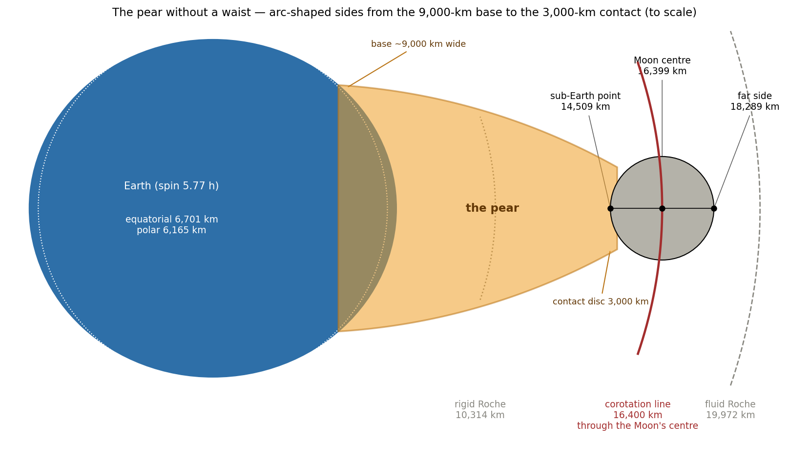
Figure 1 shows the proportions to scale: the pear’s broad base on the Earth, the single arc of its sides, and the Moon at its tip with its centre on the corotation line. The day of 5.77 h used in the drawing is the day at release, computed in §A.4.
A.4 The offset: two processes acting together
Before the Earth day at release can be calculated, two processes that act on the Earth’s spin at the same time, and in opposite directions, must both be taken into account. This matters because the day at release fixes the position of the corotation line, and therefore where the Moon is let go.
1. The pear lengthens. Material moves outward with the rotation and carries angular momentum with it; the angular momentum that leaves the Earth slows its spin. A child walking outward on a roundabout slows the roundabout in the same way.
2. The core centralises. Differentiation is the separation of an initially mixed body into layers by density: iron, the densest component, sinks toward the centre and forms a core, while lighter material is left above it. In the LEF model this organisation of the core is one continuous process: it had begun before the transfer, it continued while the pear grew, and it went on after release. Fast rotation speeds up differentiation: iron sinks inward and the Earth’s moment of inertia falls, because mass moves closer to the axis. With less moment of inertia and the same angular momentum, the body must turn faster. As with a skater drawing in her arms, the spin speeds up.
Angular momentum is conserved, and the two processes offset each other: the result is the offset between them. A calculation that takes only one of them into account does not describe the Earth of that time — the pear alone would give too long a day, and the core alone too short a one.
| Process | Effect on the day | Effect on the corotation line |
|---|---|---|
| 1. The pear lengthens | h (alone: 5.50 6.44 h) | outward (alone: 15,818 17,569 km) |
| 2. The core centralises () | h | inward |
| Both together | 5.50 5.77 h | 15,818 16,331 km |
The table reads row by row. The pear alone would lengthen the day by 0.94 h and push the corotation line outward by about 1,750 km, because a slower spin needs a larger distance before rotation supplies orbital speed. The centralising core takes back 0.67 h. Together, the day lengthens by only 0.27 h, from 5.50 to 5.77 h, and the line moves out only modestly, to 16,331 km.
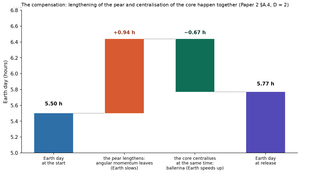
Figure 2 shows the same balance graphically: the bar added by the pear and the bar removed by the core, with the net result between them.
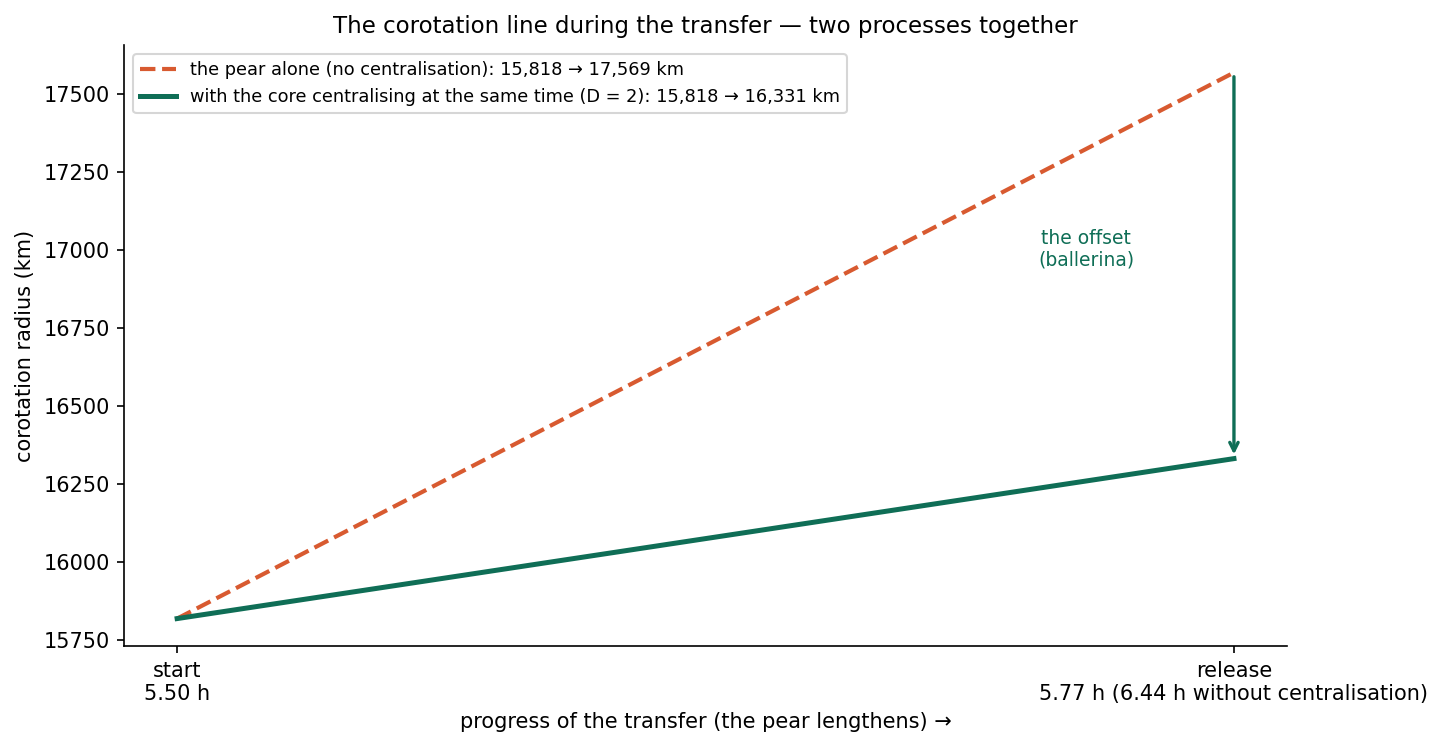
Figure 3 follows the corotation line as the transfer proceeds. With the pear alone the line runs steadily outward; with the core centralising at the same time it stays much closer to its starting position.
A.4.1 The effect of differentiation on the final state
Concentration of mass inward changes the moment of inertia. To test this, the two layer boundaries, the density, the shape and the spin were computed together. This extends the sensitivity test, and does not merely replace inside a fixed homogeneous figure: a body that differentiates also changes its flattening, and the flattening in turn changes the moment of inertia, so all four must be solved at once. The boundaries were allowed to depart from spheroids; the limitation of the spheroidal assumption in layered systems is also discussed in the literature [5].
The structure is described by two numbers. The volumetric radius ratio is the radius of the inner layer divided by the radius of the whole body; places the boundary a little beyond half-way out, comparable to the present Earth’s core. The density ratio says how much denser the inner layer is than the outer: is a uniform body, an inner layer twice as dense as the outer. The larger , the more mass sits near the centre and the smaller the coefficient (for and , ; §B.6). For a volumetric radius ratio , and a density ratio , the test-particle approximation gives:
| D | Final period, hours | Corotation radius, km |
|---|---|---|
| 1 | 6.438 | 17,569 |
| 1.5 | 6.077 | 16,907 |
| 2 | 5.770 | 16,331 |
| 2.5 | 5.505 | 15,827 |
| 3 | 5.274 | 15,382 |
The table shows one steady trend: as rises from 1 to 3, the final day shortens from 6.438 to 5.274 hours and the corotation line moves inward from 17,569 to 15,382 km. The first row, , is the pear acting alone (no centralisation); the row is the adopted state of §A.4. At the centralising core almost exactly cancels the slowing caused by the pear, and the day returns to about its starting value.
Differentiation in the final structure can offset part of the spin-down that accompanies the transfer. The rows are possible states, not a sequence of evolution in time. All rows use the same initial budget for a homogeneous parent; they do not establish that a concentrated initial structure would provide that budget. The assumptions, the full scan and the convergence checks are in Appendix C and in the calculation document linked to it.
A.5 Corotation
This section derives the corotation radius used throughout, and states where its use is valid.
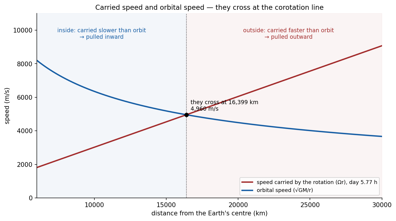
Figure 4 plots the two speeds of §A.1.3 against distance from the Earth’s centre. The speed carried by the rotation rises in a straight line; the orbital speed falls. Inside the crossing, the rotation gives less than an orbit needs and material is pulled inward; outside it, the rotation gives more than an orbit needs and material tends outward. The crossing is the corotation line.
Corotation acts on the centre of mass, not on the geometric centre, because the balance of gravity and rotation applies to the body as a whole, and the whole body moves as if its mass were gathered at its centre of mass. The corotation forces may have pulled the Moon slightly after its geometric centre crossed the line, because its centre of mass is displaced slightly toward the Earth (today about 2 km): the geometric centre reaches the line first, and the centre of mass a little later; the Moon is released slightly after its centre of mass crosses, about 210 km beyond the line (§D.3; Paper 3, §C.5a).
A.5.1 The derivation
In the test-particle approximation, in the equatorial plane and in a central field, the speed carried by the rotation is the angular velocity times the distance; the circular orbital speed follows from setting the gravitational pull equal to the force needed to keep a mass on a circle of radius :
The mass of the orbiting body cancels: the orbital speed at a given distance is the same for a grain and for a Moon. Equating the speeds gives:
Solving for , and writing :
The result says that the corotation radius depends only on the mass of the central body and on its rotation period, and grows as the period to the power two-thirds: a slower spin pushes the line outward. This is why the lengthening pear moves the line out and the centralising core brings it back (§A.4).
For a positive, constant mass and angular velocity there is a single positive root. This is the synchronous-orbit relation of standard orbital mechanics — the same relation that places geostationary satellites above today’s Earth; what is new is where it is evaluated. The classical objection evaluated the speed condition at the parent’s surface; the LEF route evaluates it at the corotation radius.
A.5.2 The release condition and the domain of validity
The equality fits an equatorial circular orbit when the radial velocity is zero and the contact forces cease — that is, when the body is moving purely sideways and the connection no longer pushes or pulls on it. With additional velocity, or with release off the equator, the initial-condition vectors must be computed. The orbital detail belongs to Paper 4; in this paper only the correction needed for the angular-momentum budget is kept, in §A.6 and Appendix D.
Reaching corotation does not cancel the work required for the lift or the transfer of angular momentum: the speed condition is met at the line, but energy and angular momentum still have to be delivered to the material on the way. The field of a flattened parent, the size of the developing body and two-body gravity also place corrections on the central description. The solution in §A.4 includes a particular two-body correction, but is not a full solution of two deformed figures connected to each other.
A.5.3 The meaning of the condition for release
The coupled solution in §A.4 defines a budgetary end state: how much angular momentum is in the Earth’s spin and how much in the Moon’s orbit at the moment of release. It does not by itself determine the onset of recession from it. An added radial velocity is also not a sufficient condition for sustained recession, because it changes the eccentricity (how elongated the orbit is) and the tides. The lag model and the rheology (the description of how the material deforms and flows under load) must be mutually consistent [3,4]. The direction of the tidal push on each side of the line is set out in §A.8.
A.5.4 The boundary between Paper 2 and Paper 4
Paper 2 fixes the mass, the spin and the budget to be handed to the orbital test. Paper 4 treats the orbital elements, the tilt and the evolution after release. There is no computed recession time here, and no general prohibition on a free orbit inside the corotation radius. In the connected scenario the free-body equations are to be replaced by the equations of the connected state where the free-body equations cease to apply: while the Moon is still attached through the pear, it is held by the connection and is not a free body.
A.6The angular-momentum budget
The speed problem is solved at the corotation radius. The second question of §A.1.1 remains: does the parent hold enough angular momentum to put the Moon there and still match the system we see today? This section builds the budget step by step: the parent’s initial angular momentum, the cost of moving the material out, the comparison with the present system, the sensitivity to period, expansion and structure, and the comparison with the classical fission route.
A.6.1The parent and the initial budget
The initial parent mass is . The material to be transferred later is still included in its moment of inertia. The parent is described as a Maclaurin spheroid: the equilibrium shape of a uniform fluid body in steady rotation, flattened at the poles and bulging at the equator, symmetric about its axis. The faster it spins, the flatter it is. In the homogeneous Maclaurin model, under the assumptions of the table, one obtains [1]:
The first line is the moment of inertia of a uniform spheroid () with the equatorial radius 6,721 km; the second multiplies it by the angular velocity of the 5.5-hour day. The result, , is the whole angular-momentum budget the route has to work with. The shape equation and the full substitution are kept in Appendix B. Uniformity is the reference assumption; a change of structure is tested below.
A.6.2 The cost of the transfer in the base calculation
Before the transfer, the lunar material is part of the parent and turns with it, carrying its share of the parent’s angular momentum. For material representing the uniform mass distribution, its mean squared distance from the axis is the same as the parent’s, and its share is:
Here is the average, over the material, of the squared distance from the spin axis. Once the same mass sits at the corotation radius and still turns with the parent, its angular momentum is:
about fourteen times more, because the distance from the axis has grown and enters squared. The difference between the two must be supplied by the parent’s spin. As a fraction of the whole budget:
About one sixth of the parent’s angular momentum is handed to the material during the transfer. This is the amount by which the parent’s spin is slowed by the pear (§A.4) before the centralising core is taken into account.
In the base calculation, an equatorial surface source gives about 13.8%; a representative sample of a similar interior region at half the original radius gives about 16.5%. The source matters because material that starts far from the axis already carries more angular momentum and needs less added. A specific interior source requires its own mean squared distance. The word “interior” must not be taken to imply that the global mean necessarily applies.
A.6.3 Comparison with the present system
The parent’s budget must now be compared with what the Earth–Moon system holds today. The present total has two parts: the Earth’s spin and the Moon’s orbit. The reference constants copied from the source give:
where m and . The second formula is the orbital angular momentum of two bodies circling their common centre: is the reduced mass, the semi-major axis of the lunar orbit and its eccentricity. The sum of the magnitudes is about , of which about 83% is orbital: most of the system’s angular momentum now lies in the Moon’s orbit, not in the Earth’s spin. The surplus of the parent’s budget relative to the sum of magnitudes is about 0.7%. The parent held slightly more than the system holds today, which is the sign required by the small loss to solar tides (§A.2).
The spin and the orbital angular momentum are vectors, and they do not point the same way: the Earth’s axis is tilted against the plane of the lunar orbit. If the angle between the vectors is , the total magnitude is:
Adding two arrows at an angle gives a shorter total than laying them end to end, so the vector total is smaller than the scalar sum and the parent’s surplus over it is larger. For the test angles 18.3°, 23.4° and 28.6° one obtains surpluses of about 1.46%, 1.92% and 2.51%. The angles serve as a sensitivity test; no observational epoch was chosen here and no full vector history was computed. The Moon’s present spin is very small, but its early spin was larger, and the two must be kept apart.
The surplus depends on how uniform the parent was. At fixed figure, varying gives a threshold of about 0.397 against the scalar sum and about 0.390–0.394 against the vector range: with below this value the parent’s budget would fall short of today’s. The present differentiated Earth has of about 0.33, well below the threshold, so the route requires that the parent was still at an early stage of sorting when the transfer began; this requirement is listed in §D.3. This is a sensitivity condition, not a stratified Maclaurin family of solutions. The positive surplus means that this test finds no angular-momentum deficit, but matching the rate of loss to the Sun requires a further calculation.
A.6.4 Sensitivity to period and expansion
A shorter initial day means more angular momentum; a larger (more expanded) parent has a larger moment of inertia and holds the same angular momentum at a longer day. The admissible initial period therefore depends on the adopted expansion. In the reference model, the window 4.90–5.54 hours refers to the initial period and to the adopted budget and loss conditions: at 5.54 hours the parent holds exactly today’s angular momentum, and at 4.90 hours it holds about 15% more, the adopted limit for loss to the outside. Its ceiling must not be applied to the final period after the transfer of angular momentum, which is longer by design (§A.4). Appendix B retains the original sensitivity table, with the distinction between an adopted expansion and a thermal calculation not yet performed.
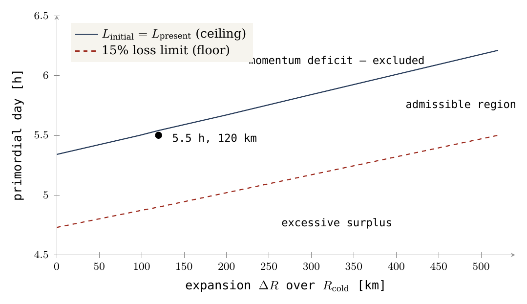
Figure 5 is read as a map of allowed starting states. The horizontal axis is how much the hot parent was expanded over its cold radius; the vertical axis is its day. A starting state above the solid line holds less angular momentum than today’s system and is excluded; a state below the dashed line holds more than 15% extra, more than the outside loss can remove. The band between them is admissible, and it rises to the right because a larger parent holds the same angular momentum at a longer day. The reference state, 5.5 h with 120 km of expansion, lies inside the band, just below the ceiling.
A.6.5 Comparison of equilibrium figures
The classical objection to fission can now be placed exactly. In the classical route the whole Earth must spin so fast that it becomes unstable and divides. A uniform rotating fluid follows a known sequence of shapes as its angular momentum grows. At first it is a Maclaurin spheroid (§A.6.1), flattened but round in the equator. At a definite flattening a second family branches off: the Jacobi ellipsoids, whose equator is no longer a circle but an ellipse, so the body becomes elongated like a rugby ball turning end over end. Further along the Jacobi sequence comes a pear-shaped figure, from which classical fission was expected to proceed. Each of these points requires a definite spin and a definite angular momentum.
At the classical bifurcation point from Maclaurin to Jacobi, with and , one obtains for the adopted mass and volume hours, km and an angular momentum of about , a ratio of about 2.74 to the present sum [1]. Here is the eccentricity of the meridian section (zero for a sphere, approaching one for a very flat body) and measures the spin against the body’s own gravity. In plain terms: merely to reach the first step of the classical path, the Earth would need a day of under three hours and almost three times the angular momentum the Earth–Moon system holds.
This is a comparison with a defined configuration on this classical path. The value 4.08 of the original reference calculation refers to a different point on the Maclaurin sequence — the maximum- point, not the Jacobi bifurcation — and is not presented as a universal bound. It is the source of the familiar statement that fission needs about four times too much angular momentum. The value 3.5 for the pear-shaped point is not adopted because verification of the table has not been completed.
The reason for the difference is the place where the speed condition is evaluated. The classical route asks the parent’s surface to reach orbital speed (§A.1.2); that forces the parent towards break-up, and break-up costs several times the available angular momentum. The LEF route never uses that condition: the material is carried out in corotation and the speed match is made at the corotation radius (§A.5), where a parent turning once in 5.5 hours already supplies orbital speed. Evaluated there, the requirement falls to the budget the parent actually has. The comparison is between two routes to the same product: the classical one needs 2.74 times the present budget; this one needs 1.007.
A.6.6 The vector correction for release off the equator
So far the material was assumed to leave in the equatorial plane. Off the equator the spin vector and the orbital angular momentum must be summed in the same frame, because the orbit of a body released at a latitude is tilted against the spin. Let be the spin angular momentum and the orbital angular momentum of the released body, where is the angle of release from the equatorial plane. For the geometry defined in Appendix D:
This is the same rule for adding two arrows at an angle as in §A.6.3: the initial budget must equal the vector sum of the spin and the tilted orbit.
In the example relative to the final axis and a homogeneous structure, the two-mass coupled calculation gives a final period of 6.220 hours, a reference distance of about 17,240 km and an orbital angular momentum of about 15.83% of the budget. The 25° value is a sensitivity test of how much an off-equator release changes the budget; the adopted release latitude, the centre of the contact area, is 22.5° (Paper 4). This is a sensitivity correction to the budget, not a newly adopted reference value. The derivation of the inclination and eccentricity, the perigee and the evolution after release are handed to Paper 4.
A.6.7The budgetary decision condition
The test requires a consistent initial state, final state and external transfer:
The equation is conservation of angular momentum written as an account: what the system started with equals what it holds now plus what was removed from outside (for the Earth–Moon system, chiefly by the Sun’s tide). Closing the numerical balance proves consistency between the states defined. Failure to find a match within the supported ranges of structure and external transfers would rule out this budgetary scenario. A match does not establish how the body mechanically reaches the final state; that is the subject of Paper 3.
The budget therefore stands as follows: the parent of 5.5 hours holds slightly more angular momentum than today’s system, the transfer costs about one sixth of it, and the classical route would have needed 2.74 times as much.
A.7The Roche limit
A body that reaches the corotation radius must also hold together there. Close to a massive parent, the parent’s gravity pulls harder on the near side of the body than on the far side; this difference, the tidal force, tends to stretch the body apart. The Roche limit is the distance inside which this stretching exceeds the body’s own gravity holding it together. A body held only by its own gravity cannot remain whole inside it.
A.7.1Two reference limits
For and the parent mass after departure:
(An earlier version gave 10,313 km; the two are the same within rounding, and the series uses 10,314 km. Figures 1, 6, 8 and 9 print the fluid limit as 19,972 km, the same value within rounding.) The bracketed term is the radius a sphere of the Earth’s mass would have if it had the satellite’s density; the limit is a fixed multiple of it. The two formulas differ only in that multiple, and the reason is physical. The fluid approximation concerns a deforming body: as it is stretched it lengthens toward the parent, its near and far ends move farther apart, the tidal difference across it grows, and it gives way sooner — so the fluid limit lies farther out. The so-called rigid approximation neglects the change of shape: the body keeps its round form, the tidal difference across it stays smaller, and it survives closer in. It contains no crustal thickness or material strength [1]; it is a body held by its own gravity alone that merely does not change its shape. The base radius and the two coupled radii lie between these limits: inside the fluid limit, outside the rigid one. The presence of a crust alone therefore does not establish survival; survival depends on whether the body behaves as rigid on the time-scale it spends there.
The Roche limits move inward as the body density increases, because a denser body holds itself together more strongly. A density of about 4,700 kg per cubic metre would move the fluid limit to the release distance of about 16,400 km; for the rigid body at release the rigid limit applies (§B.7). This is a requirement computed in the Roche approximation, not evidence that the body reached that density or a solution to all the stability requirements.
A.7.2 What the comparison of accelerations teaches
The basic comparison is between the parent’s gravity gradient and the self-gravity:
The first quantity, , is the difference between the parent’s pull at the body’s centre and at its surface, a distance closer; it falls steeply, as the cube of the distance . The second, , is the body’s own surface gravity holding its material in. When the first is smaller than the second, the body’s own gravity wins. With the reference data of Appendix E the ratio is below unity (about 0.277 at 15,818 km). This is a useful measure of loading, but change of shape and rotation are not included in the ratio. The static Roche limit provides a basis for comparison; the response in an eccentric orbit may also depend on the deformation history [9].
A.7.3What remains conditional
The corotation radius is not a strength threshold: reaching it settles the speed, not the survival. The properties of the body and of the connection are examined in Paper 3, and the orbit after release in Paper 4. Paper 2 adopts no binding residence time in the Roche domain and no universal viscosity threshold. The comparison should use the closest distance of the chosen orbit, not the release distance alone. Dividing the tests among the papers does not remove the requirement of survival.
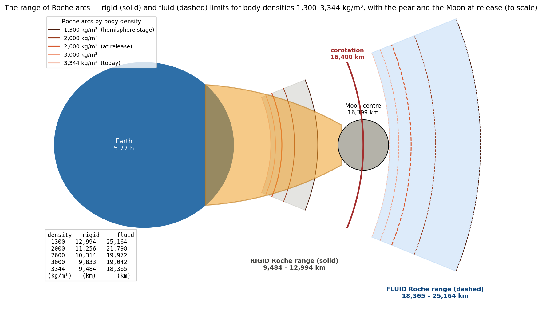
Figure 6 places the Moon at release against the two families of limits. The rigid limits for the whole range of densities lie well inside the Moon’s position; the fluid limits lie beyond it. The Moon at release is therefore safe as a rigid body, and its flattening and rounding were completed earlier, while it was still attached (§B.7; Paper 7).
A.8The direction of tidal evolution
The last question of Part A is what happens after release: does the Moon move away from the Earth or fall back? The answer depends on which side of the corotation line it lies.
A.8.1 The direction of angular-momentum transfer
For a direct, circular, equatorial orbit, we compare the parent’s spin with the mean motion — the angular velocity of the orbiting body around the parent:
The orbiting body raises a tidal bulge on the parent. When , the parent turns faster than the body orbits, and its rotation carries the bulge ahead of the body; the bulge pulls the body forward, gives it angular momentum, and the body climbs outward while the parent’s spin slows. In the language of the tidal equations, the dissipative tidal contribution in the parent transfers angular momentum from its spin to the orbit. When , the body outruns the bulge, the bulge pulls it back, and the direction reverses: the body loses angular momentum and spirals inward. At exact circular synchronism the relevant contribution vanishes: the bulge stays directly beneath the body and there is no forward or backward pull. Since falls with distance and does not, holds outside the corotation radius and inside it. The corotation line is thus a watershed: a body released just beyond it is pushed outward from the start. Generalisation to an orbit with inclination and eccentricity requires the appropriate tidal equations [2,3].
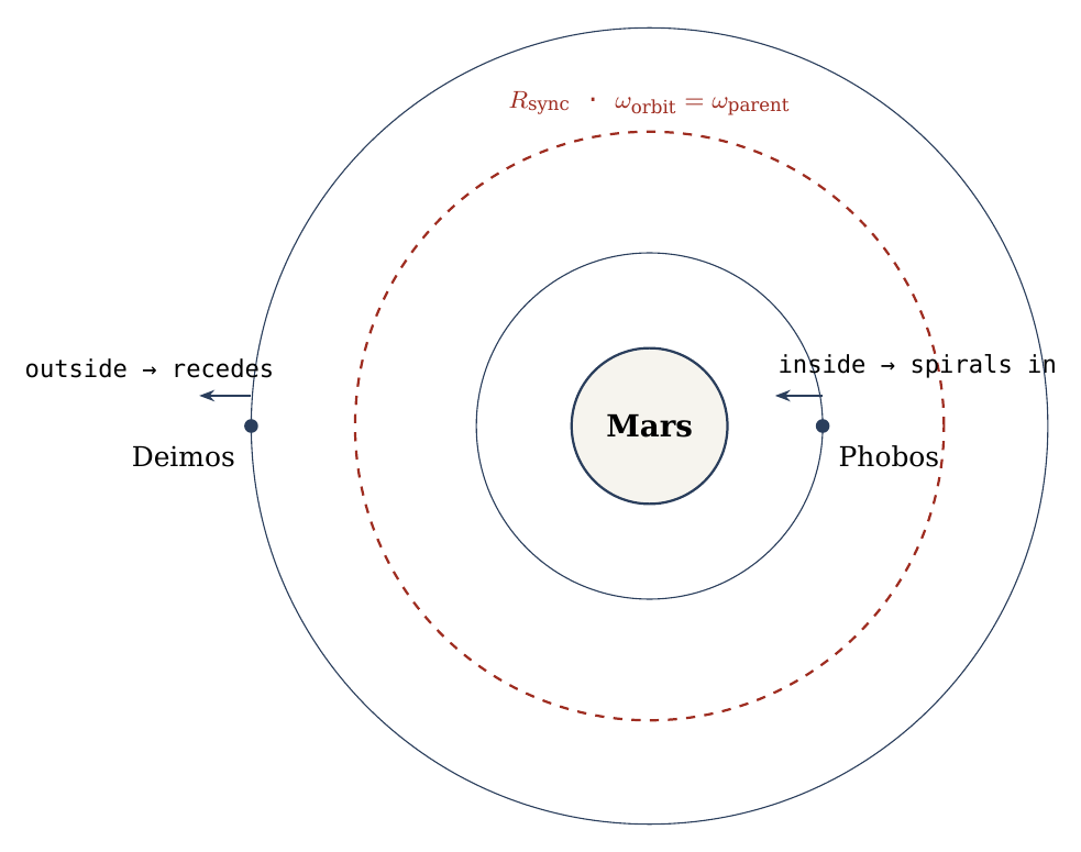
Figure 7 shows the watershed at work in the present Solar System. Mars has two small moons on opposite sides of its synchronous radius: Phobos, inside, is being drawn inward; Deimos, outside, is moving away. The Earth–Moon case at release is the same rule applied to a Moon placed just beyond the line.
With Part A complete, the problems are fully defined: a velocity gap that closes at the corotation radius, a pear that reaches that radius, a day at release set by two opposing processes, a budget that must close against today’s system, a Roche test the body must pass, and a tidal watershed that decides its later direction. Part B answers them with one calculation.
How the problems are solved
One calculation answers the problems of Part A. Section B.1 sets out that calculation from its inputs to the state of the Earth and the Moon at the moment of release. Each subsequent section (B.2–B.8) takes one problem of Part A, in the same order, and states in two or three sentences how the calculation meets it.
Part A stated the conditions; this Part shows that a single, consistent set of numbers meets all of them at once. The point matters because each condition taken alone can usually be met by tuning one parameter, while meeting all of them with the same Earth, the same Moon and the same spin is a much stronger test of the route.
B.1The calculation
Inputs. Initial Earth day h (§A.2); a homogeneous, expanded parent of volumetric radius 6,517 km and density 5,214 kg m (equatorial 6,721 km, polar 6,128 km); the Moon: one lunar mass, kg, density 2,600 kg m. “Homogeneous” means that the parent is taken as uniform in density at the start, a calculation input for a parent still at an early stage of sorting; “expanded” means that it is hot and therefore somewhat larger than a cold Earth of the same mass (§A.2). The equatorial and polar radii differ because a body spinning once in 5.5 h bulges at the equator and flattens at the poles.
From Part A to the release state, step by step. The release state follows from the processes of Part A in five steps. The table below collects them; its rows are read from top to bottom, and the tint shows the direction of each step: red for a step that slows the Earth and moves the corotation line outward, blue for a step that speeds it and moves the line inward.
The starting point. A parent with a 5.5-h day has its corotation line at 15,818 km (§A.2.1). The corotation line is the distance at which a body turning together with the Earth already moves at the speed of a free circular orbit.
The pear slows the Earth. As the pear lengthens, material moves outward while still turning with the Earth, and it carries angular momentum with it. Angular momentum is the “quantity of rotation” of a body, its mass times its speed times its distance from the axis; with no outside torque its total is conserved. The angular momentum that leaves with the material is taken from the Earth’s spin, so the Earth turns more slowly: alone, this step would lengthen the day from 5.50 to 6.44 h and move the line out to 17,569 km (§A.4).
The organising core speeds the Earth. At the same time iron sinks toward the centre. This lowers the Earth’s moment of inertia — the measure of how far its mass lies from the axis — and, like a skater drawing in her arms, the Earth turns faster. With a core twice as dense as the mantle above it (), this step removes 0.67 h from the day.
The net result. The two steps act together and partly cancel: the day at release is 5.77 h, and the corotation line lies at 16,331 km when the Moon is treated as a test particle, or 16,399 km when the Moon’s own mass is included in the two-body formula below. We use the two-body value, rounded to about 16,400 km.
Release. The Moon begins to separate when its centre of mass reaches this line. It is carried there by the rotation, not thrown: at that distance the speed it already has as part of the turning system is the speed of a free orbit, so no extra push is required (§B.2).
| Step | Earth day | Corotation line | Direction |
|---|---|---|---|
| 1. Start (5.5-h parent, §A.2.1) | 5.50 h | 15,818 km | reference |
| 2. The pear lengthens (alone) | 6.44 h | 17,569 km | slower, line outward |
| 3. The core organises () | h | — | faster, line inward |
| 4. Both together (test particle) | 5.77 h | 16,331 km | net: slightly slower |
| 4a. Both together (two-body) | 5.77 h | 16,399 km 16,400 km | adopted |
| 5. Moon’s centre of mass on the line | 5.77 h | 16,400 km | release |
The quantitative content of these steps is the following.
1. The Earth day at release. The lengthening pear and the centralising core act together (§A.4); with , Here is the length of the day and the angular velocity of the spin, the angle in radians turned per second. The day is only about a quarter of an hour longer than the starting 5.5 h, because the speed-up from the sinking iron cancels most of the slow-down caused by the pear.
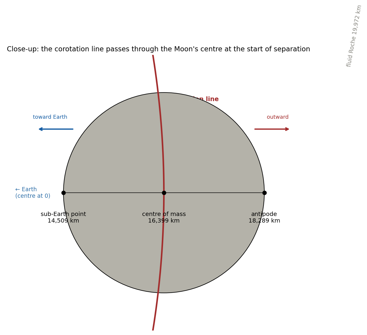
2. The release point. The Moon begins to separate when its centre of mass reaches the corotation line: This is the corotation formula of §A.5.1, written for two bodies: is the gravitational constant, the Earth’s mass and the Moon’s. In words, it gives the one distance at which a circular orbit takes exactly as long as one turn of the Earth. Including in the formula is what turns 16,331 km into 16,399 km. The value is about 2.6 times today’s Earth radius. With km, the near point lies at 14,509 km and the far side at 18,289 km from the Earth’s centre. is the radius of a sphere of one lunar mass at a density of 2,600 kg m; subtracting and adding it to the 16,400 km of the centre gives the extent of the Moon along the Earth–Moon line.
3. The Earth at release (Maclaurin, homogeneous): A Maclaurin spheroid is the equilibrium shape of a uniform fluid body spinning steadily: a sphere flattened at the poles. The equation links the spin (left side, with the Earth’s mean density) to the eccentricity , a number that measures the flattening (0 for a sphere, approaching 1 for a flat disc). Solving it for the 5.77-h spin gives the equatorial radius and the polar radius . The Earth at release is thus still clearly flattened, though slightly less than the 5.5-h parent (6,721 and 6,128 km), because it now turns a little more slowly. The gap between the Earth’s equatorial surface and the Moon is about 7,800 km: the Moon’s near point at 14,509 km less the equatorial radius of 6,701 km. This is the distance the pear has to bridge (§A.3).
4. The angular momentum. The first expression is the starting budget of the parent (§A.6.1, in kg m s): the moment-of-inertia coefficient (0.4 for a uniform body), the mass, the square of the equatorial radius and the initial spin. The second expression divides the same budget at release into two parts: the Earth’s spin, , where is its moment of inertia, and the Moon’s orbit, , where is the reduced mass of the pair and the release distance. At release the Moon’s orbit holds (17%) and the Earth’s spin ; the system holds 1.007 times today’s value (an earlier version gave 1.008, from today’s total rounded to ; with of §A.6.3 it is 1.007, the value used throughout). The is defined as the orbital angular momentum of the pair about their common centre, , with the reduced mass kg and km on the equator. Counting the full lunar mass about the Earth’s centre, as Paper 3 does, the same state gives ; for release at 22.5 ( km, Paper 4), where the Moon turns at km from the spin axis, the same count gives (Paper 3). The 17% is the price of the transfer: the share of the original rotation that has moved from the Earth’s spin into the Moon’s orbit. The total, 1.007 times today’s, is slightly above the present value, which is the sign required, since solar tides have removed about 1% of the system’s angular momentum since then (§A.2).
Earth day at release 5.77 h; Moon centre at 16,400 km; angular momentum 1.007 times today’s.
Figure 8 draws this state to scale. It shows how close the Moon still is to the Earth at release: the gap of about 7,800 km is spanned by the pear of §A.3.
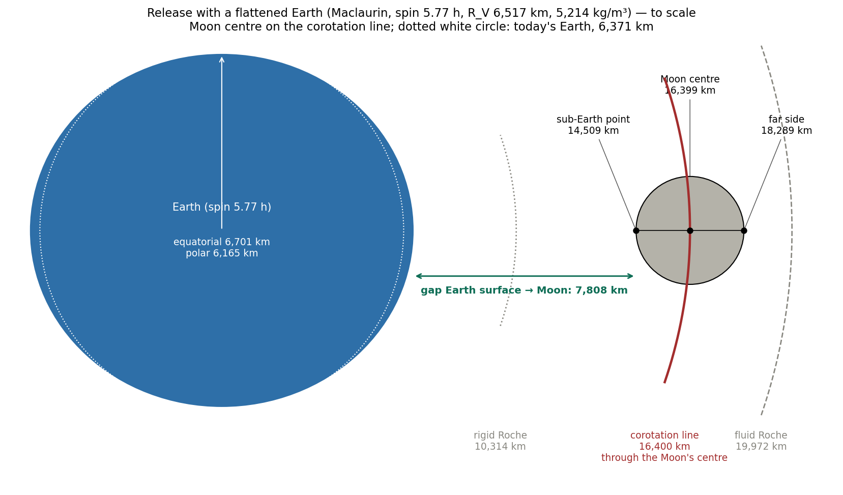
What we now have is a complete release state: the Earth’s day and shape, the Moon’s position and size, and the division of the angular momentum between them. The following sections check this state against each problem of Part A.
B.2The velocity gap
The problem of §A.1 was that material released from the surface of a 5.5-h Earth moves at about 2,133 m s, far below the 7,701 m s of a circular orbit, a gap of about 5,568 m s. The gap closes with distance, because the speed carried by the rotation grows with distance while the orbital speed falls. On the corotation line the rotation gives the Moon exactly the orbital speed, so no gap remains (§A.1, §A.5). The left side is the speed of a point turning with the Earth at distance ; the right side is the speed of a free circular orbit at the same distance; on the line they are equal. The value is a little below the 5,020 m s of the 5.5-h reference (§A.2.1), because the slightly slower Earth places the line farther out, where orbital speeds are lower. The everyday picture is a child on a roundabout: the farther from the centre she sits, the faster she moves, without anyone pushing her.
B.3The pear
The pear bridges about 7,800 km and lies entirely inside the corotation line; the Moon is released when its centre of mass reaches the line (§A.3; the mechanism of release is Paper 3, LEF Mechanism in Practice). Because the pear lies inside the line, the net force in the turning frame pulls it toward the Earth (§B.5): it stays with the Earth, while the Moon, whose centre is on the line, is free to separate. This is why the Moon leaves whole and the connection does not go with it.
B.4The offset
The calculation takes both processes into account together: Earth day 5.77 h, corotation line 16,331 km (§A.4). The 16,331 km is the test-particle value of step 4 in §B.1; including the Moon’s own mass gives the 16,399 km, about 16,400 km, used for the release point. A calculation with the pear alone would give 6.44 h and 17,569 km, and one with the core alone would give too fast an Earth; only the two together describe the Earth of that time.
B.5 Corotation
The Moon’s centre of mass reaches the corotation line at about 16,400 km; beyond it corotation pulls the Moon outward and it is released: This is the net acceleration felt by material that turns with the Earth at distance , seen in the turning frame. The first term is the outward (centrifugal) acceleration of the rotation, which grows with distance; the second is the Earth’s gravity, which falls with distance. Inside the line gravity wins and points inward, which is why the pear is held to the Earth; on the line the two balance; beyond it the rotation wins and the material is drawn outward. As soon as the Moon’s centre of mass passes the line, the body as a whole is drawn away from the Earth, and it separates.
Figure 9 enlarges the moment at which separation begins. The line is drawn through the Moon’s centre; the near half of the Moon still lies inside it and the far half outside.
B.6 The angular momentum
The system holds 1.007 times today’s angular momentum. At release the Earth’s moment-of-inertia coefficient implied by its remaining spin angular momentum is ; a two-layer structure with and gives The coefficient describes how the mass is distributed: 0.4 for a uniform sphere, lower when mass is gathered toward the centre (today’s Earth has about 0.33). The value 0.355 is what the Earth must have at release if its spin of 5.77 h is to carry the remaining . The formula computes for an Earth of two layers: an inner layer reaching to a fraction of the radius, with a density times that of the outer layer. With and it gives 0.360, close to the required 0.355. The angular momentum demanded by the release state and the structure produced by the sinking iron thus agree with each other. No giant impact from outside and no later removal of angular momentum are needed; high-angular-momentum impact models start at about 2–3 times today’s value. The route closes its budget with what the Earth–Moon system holds today plus the roughly 1% that solar tides have since removed.
B.7The Roche limit
The Roche limit is the distance inside which the tidal pull of a large body, the difference of its gravity between the near and the far side of a smaller body, exceeds the smaller body’s own gravity and can pull it apart. Two classical forms bound it: The rigid form applies to a body that keeps its shape; the fluid form to a body that deforms freely and so is stretched further by the tide. In both, is the density of the small body: the denser it is, the closer it can come. The Moon’s centre at 16,400 km lies well beyond the rigid limit (9,484–12,994 km for 1,300–3,344 kg m). The same distance lies inside the fluid limit for a body of 2,600 kg m (19,971 km, §A.7.1); which of the two limits applies is therefore decided by whether the Moon is rigid at release. The rounding was completed before release; the body is rigid and round. The flattening and the later rounding of the lunar body took place earlier, while it was still attached (Paper 7, The Poles); what leaves the line is a body with a rigid outer shell. A rigid body reduces the tidal response by so that for GPa the axis ratio is at most 1.04. Here is the rigidity (shear modulus) of the body, its surface gravity and its radius; is the pressure of the body’s own weight. The factor says that a body whose rigidity is large compared with the pressure of its own weight deforms only a small fraction of what a fluid body would. An axis ratio of at most 1.04 means that the longest axis of the Moon exceeds the shortest by no more than 4%: the body remains round.
B.8The direction of tidal evolution
The Moon is released on the corotation line, and tides transfer angular momentum to it from the Earth’s spin: it recedes (§A.8; the orbit is Paper 4, The Orbit). Exactly on the line the tidal effect is neutral, since the Earth turns once in the same time as the Moon orbits. Separation itself carries the Moon’s centre of mass about 210 km beyond the line, when a little more than half of the Moon has crossed it (the margin of §D.3); there the Earth spins faster than the Moon orbits, the tidal bulge raised on the Earth runs ahead of the Moon, pulls it forward, and the Moon moves outward. This is the side of the watershed on which Deimos lies today (Figure 7).
How far beyond the line. The distance beyond the line is small against the release radius, but it sets the shape of the first orbit. On the line the Moon carries exactly the speed of a circular orbit; beyond it, a little more, so the release point becomes the nearest point of a slightly stretched orbit, with an eccentricity that grows with the distance. The table follows this at the release latitude of 22.5°, where the corotation line lies at 17,287 km, with the 5.77-hour day; the initial orbit comes from the formulas of Paper 4 (Appendix A) and the final angle from the reduced tan-law of Paper 4 (Part D). “Crossed” is the share of the Moon’s volume beyond the line at release.
| Offset (km) | Crossed | (km) | Final angle | |
|---|---|---|---|---|
| 0 | 50% | 17,287 | 0 | 5.020° |
| 50 | 52% | 17,489 | 0.009 | 5.049° |
| 100 | 54% | 17,696 | 0.017 | 5.079° |
| 150 | 56% | 17,907 | 0.026 | 5.109° |
| 210 (adopted) | 58% | 18,163 | 0.037 | 5.145° (observed) |
| 300 | 62% | 18,571 | 0.053 | 5.202° |
| 500 | 69% | 19,531 | 0.089 | 5.334° |
| 1,000 | 86% | 22,404 | 0.184 | 5.711° |
Table B.8. Release at 22.5°: the initial orbit and the final angle of the reduced law as the release moves beyond the corotation line (Paper 3, §C.5a). The navy deepens with the final angle; green marks the observed 5.145°, which is the adopted release.
Release exactly on the line gives a circle, and the tide carries a circle outward as a circle; the Moon’s present eccentricity therefore requires a release a little after its centre of mass has crossed. At about 210 km the reduced law returns the observed inclination, and Paper 3 (§C.5a) shows that the same offset returns today’s eccentricity of 0.0549 for a hot young Moon; the series adopts this release. Paper 3 gives the eccentricity table and the sensitivity to the latitude of the tip; the full integration of Paper 4 carries the release state through the whole history.
What we now have: the release state of §B.1 meets each of the seven problems of Part A with one set of numbers.
Summary
C.1 What has been shown
The table pairs each problem of Part A with the answer given in Part B. It is read row by row; each check mark means that the release state of §B.1 meets that problem without a separate assumption.
| Problem | Solution | |
|---|---|---|
| The velocity gap | the speed comes from the rotation; on the line there is no gap | |
| The pear | bridges to the line; the Moon is released whole | |
| The offset | 5.77 h — both processes together | |
| Corotation | centre of mass on the line, 16,400 km | |
| Angular momentum | 1.007 times today’s; consistent with the core structure | |
| The Roche limit | rigid body, well beyond the rigid limit | |
| Tidal evolution | recedes from release |
Claims, tests, requirements and novelty
This Part collects in one place what the paper claims, how each claim is tested, and what the route requires of its mechanism, so that these points are found here rather than scattered through the text.
Core centralisation during the transfer. The organisation of the core is one continuous process: it had begun before the transfer, it proceeds while the pear grows, and it goes on after release. (Without the sinking iron the pear alone would slow the Earth to 6.44 h, §B.4.)
A rigid body ( GPa) at release. (A fluid body at 16,400 km would lie inside the fluid Roche limit, §B.7.)
A continuous pear from the Earth to a 3,000-km contact disc, with no neck remnant attached to the Moon. This is the condition for the Moon to leave whole; it is examined in Paper 3.
D.1Central claims and tests
The table lists the five central claims. The first column names each claim and states its status; the second, what it assumes and predicts; and the third, how it is tested.
|
Claim / status |
Assumptions and quantitative prediction | Test and sensitivity |
|---|---|---|
| Corotation — an application of standard physics | Central field, equator, defined and ; | Reproduction of the two velocities and check of field corrections |
| Closure of the angular momentum — a consistency test of the scenario | ; release with the centre of mass on the corotation line, about 16,400 km () | Reproduction of , vector budget and domain of external transfers |
| Sensitivity to structure — a computed result | A change of in the two-layer model changes and | Scan of and ; check of shape and convergence |
| Non-equatorial angular momentum — a geometric correction | Definition of relative to one axis for all vectors | Vector sum and check of all angular-momentum components |
| Survival — an open requirement | Defined density, structure and orbit | Roche comparison and deformation solution in the follow-on papers |
In plain words, the claims are these.
Corotation. The claim is that at the corotation line the speed from the rotation equals the orbital speed. The corrections the scenario needs (the flattened Earth’s field, the size of the Moon, the pull between the two bodies) are checked against that equality.
Closure of the angular momentum. The claim is that the starting budget of suffices for a release at about 16,400 km. The budget before release is matched to the budget after it through the structure and the solar-tide loss.
Sensitivity to structure. The claim is that a sinking core changes the day and the line in the computed way (§A.4.1). The calculation settles on a solution for each structure scanned.
Non-equatorial angular momentum. The claim is that a release off the equator changes the budget only by the computed vector correction (§A.6.6). All vectors are summed in one frame.
Survival. The claim is that the Moon survives the Earth’s tide at release. This is tested in the following papers.
These claims are not all independent observational predictions: some are physical identities, some consistency tests and some requirements on the mechanism. The distinction is kept in the novelty map of Appendix F. An identity, such as the corotation formula, cannot be wrong if the inputs are right; a consistency test checks that the numbers close; a requirement is a condition the next papers must meet.
D.2The novelty of the work
The corotation formula, Maclaurin figures, conservation of angular momentum and the Roche limits are prior physics. The work examines their joint application to a connected-transfer condition, with a consistent computation of the change in mass, shape and spin and a presentation of the sensitivity domains. “Connected transfer” means that the material stays joined to the Earth and turns with it until it reaches the line, instead of being launched from the surface; this is the release condition under which the classical objection to fission, a budget several times too large, does not arise (§A.6.5). A full claim of historical priority requires the prior-work check of Appendix F; the success of the numerical reproduction does not prove priority.
D.3What is assumed and required
The assumptions and requirements supporting the argument are collected here to avoid repeating them alongside each result. Each row gives the value adopted or required.
| Adopted or required | Value |
|---|---|
| Initial rotation period | 5.5 h; window 4.90–5.54 h at km |
| Thermal expansion | 120 km; admissible 98–520 km |
| Parent structure at the start of transfer | At an early stage of sorting, (calculation input); the organisation of the core is one continuous process that goes on through the transfer and after release |
| Release condition | Corotation maintained to release; release beyond the corotation radius by km ( km) |
| Survival at release | Interior viscosity of order – Pa s, or density above 4,700 kg/m, at which the fluid Roche limit reaches the release distance of 16,400 km (§A.7.1; an earlier version gave 3,800 kg/m, the value for the earlier pear-alone distance of 17,569 km) |
| The tidal watershed | Satellites outside the corotation radius recede, inside it fall |
| The budget comparison | Scalar as baseline (0.7%), vector as sensitivity (1.5–2.5%) |
A few rows need a word of explanation. The thermal expansion is the amount by which the hot young Earth was larger than a cold one; 6,495 km is the volumetric radius at the lower end of the admissible range (98 km of expansion). The release condition reads as follows. A body released exactly on the corotation line is in a tidally neutral state; as soon as it lies beyond the line, the tide pushes it outward, so the Moon recedes from the start (Paper 4, §B.2). Separation places the centre of mass beyond the line by a margin , where is the thickness scale of the connection (Appendix E, row E47); the margin is about 210 km, km, set by the release-distance search of Paper 3, §C.5a (an earlier version gave about 100 km). The budget comparison is made in two ways: summing the spin and orbital angular momenta as plain magnitudes (scalar), which gives a surplus of 0.7%, and as vectors at an angle, which gives 1.5–2.5% (an earlier version gave 1.5–2.6%; the largest of the three tested angles gives 2.51%); the scalar sum is the baseline and the vector sum a sensitivity test (§A.6.3).
The first three rows are adopted values with windows; the next two are requirements the route places on Paper 3; the last two are the checks this paper itself performs. None of the seven is hidden inside a result, and none is needed to state the corotation radius, which follows from the parent’s mass and spin alone.
Conclusions
A body the size of the Moon can reach orbit from the Earth’s own material without a giant impact from outside. A fast-spinning Earth supplies the speed; the pear connects the Earth to the corotation line; the lengthening pear and the centralising core together set the Earth day at release to 5.77 h; the Moon, rigid and round, is released when its centre of mass reaches the corotation line at about 16,400 km; the angular-momentum budget closes at 1.007 times today’s value, consistent with the loss to solar tides; and the Moon recedes from the moment of release.
Put as a single chain: the Earth’s rotation carries the material outward; the line where carried speed equals orbital speed sets where the Moon leaves; the balance of the pear and the core sets where that line is; and the angular momentum the Earth started with is enough, with about 1% to spare for the Sun to remove later.
E.1The earlier conclusions retained
The following conclusions of earlier versions of this paper remain valid and are kept here, with their original reference values.
The release condition determines the velocity test; direct release from the surface and transfer in corotation are different initial conditions. A surface release leaves a velocity gap (§A.1.2); a corotating transfer leaves none (§B.2).
The original reference value is about 15,818 km at a period of 5.5 hours and in the mass definition set for it. It is the line before the transfer began; the release value of about 16,400 km is the line after the pear and the core have acted (§B.1).
The addition to the material is about 15.6% in the base and about 16.5% in the coupled solution; about 17.7% is the final orbital angular momentum in the test-particle approximation, for the coupled state with the pear alone (, 6.44 h, 17,569 km); in the release state with the Moon’s orbit holds about 17.0% (§B.1). These three percentages measure different quantities: the first two, the angular momentum that the material must gain during the transfer (§A.6.2); the third, the share of the budget held by the Moon’s orbit at the end.
The internal structure and the vector geometry affect the result, and were therefore included as sensitivity tests and not as measured past values.
Corotation supplies the speed and the budget. Mechanical detachment beyond corotation, sustained recession and survival in the Roche domain are the three conditions the route places on its mechanism; they are collected in §D.3.
Further work — openings for research
The calculations in this paper define the inputs for further work that other research groups are equipped to undertake. Each item names a calculation this paper does not perform and the paper of the series that would use its result.
The stratified Maclaurin problem. The coupled end state (§A.6.2) uses a uniform figure at a varying inertia coefficient. A Clairaut–Darwin–Radau treatment of a parent with descending iron gives the corotation radius for the centralising core self-consistently (about 16,300–16,400 km at ), and hands Paper 4 its starting orbit. The Clairaut–Darwin–Radau method is the standard way of computing the shape of a rotating body whose density increases inward; it would replace the uniform shape used here with one that follows the sinking iron.
The dissipation of the early Earth. The recession from about 2.6 Earth radii (16,400 km; 2.8 Earth radii in the earlier pear-alone state of 6.44 h) is set by and its history; the present value is anomalous. Here measures how much the Earth deforms under a tide and how much of the tidal energy it dissipates; their ratio sets how fast the Moon recedes. Ocean-resonance models run from the 5.77-hour day of release (rather than the 6.4-hour day of the earlier, pear-alone state) would give the rate function that Paper 4 requires.
The thermal expansion of the parent. The 120 km adopted here (98–520 admissible) is an estimate from magma-ocean depth and melt expansion; an equation-of-state integration of a hot, volatile-rich early Earth would fix it and, with it, the rotation window.
The onset of recession. A body released exactly on the corotation line feels a tidally neutral state: the Earth turns once in the time the body orbits once, and the tide neither pushes it out nor pulls it in. As soon as the body lies beyond the line, the tide pushes it outward, so the Moon recedes from the start (§B.8; Paper 4, §B.2). Separation leaves the centre of mass beyond the line by the release margin , about 210 km (§D.3, §E.1). A tidal integration with a frequency-dependent rheology in both bodies, starting from the release state of Paper 3, would fix the margin’s range and the rate of the first recession. “Frequency-dependent rheology” means that the way each body yields to the tide depends on how fast the tide changes.
Survival inside the fluid Roche limit. The order-of-magnitude strain estimate of the appendix “Estimate of acceleration and strain” is not a deformation solution. A visco-elastic calculation of the rigid body of 1,890 km at about 16,400 km from the Earth, over the – years it spends there, would replace it. A visco-elastic calculation treats the body as elastic over short times and slowly flowing over long ones, which is how a hot body with a rigid outer shell behaves.
The classical route. The factor 2.74 at the Jacobi bifurcation is computed; the pear-shaped point along the Jacobi sequence requires the tabulated values to be verified, and a modern computation of the sequence for this mass and density would settle it. The Jacobi sequence is the family of elongated, three-axis equilibrium shapes into which a fast-spinning fluid body passes beyond the Maclaurin shapes (§A.6.5).
Code availability
All numerical results of this paper are reproduced by the scripts of the LEF reproduction package (Python 3, numpy, scipy), which prints the values of each section from the inputs stated in the text. The package is attached to this preprint as supplementary material (LEF_code_and_data.zip). An earlier version of the series and of the package is deposited at doi:10.5281/zenodo.22743615.
Derivation of corotation, definitions and constants
This appendix fixes the definitions on which every number of the paper rests. It supports the corotation radius of §A.2.1 and §A.5 (15,818 km for the 5.5-hour reference) and the release distance of §B.1. A reader who wants to check any result should begin here, because most apparent disagreements between reproductions come from a different choice of mass, distance or constant, not from a different physics.
The short full derivation is in §B.1. Two masses must be kept apart. is the total initial mass: the Earth and the lunar material together, before any of it has left. is the final parent mass: the Earth after the lunar material has been assigned to the second body. Using one where the other is meant counts the lunar mass twice or not at all.
Two distances must also be kept apart. A radius relative to the parent’s centre is not a radius relative to the centre of mass of the system; once a second body of real mass exists, the two bodies turn about their common centre of mass, which lies slightly away from the Earth’s centre. In the two-body case the distance is between the centres, and the gravitational parameter (the product of the gravitational constant and the mass that pulls) is , because each body orbits under the pull of the other and the relative motion is governed by the sum of the masses.
The constants are the reproduced source inputs, not a new fit to an ephemeris (a table of observed positions). Changing the definition of the mass therefore requires a new calculation, not a silent change of the label 15,818: that number belongs to one stated definition, and a different definition produces a different number.
The rotating geometry and the coupled angular-momentum budget
This appendix derives the shape and the angular momentum of the young Earth before the transfer begins. It supports the initial budget kg m s of §A.6.1 and §B.1, the comparison with the present system in §A.6.3, and the admissible region of Figure 5 in §A.6.4. The steps are: fix the mass and the size; find the flattened shape a uniform body takes at a 5.5-hour spin; compute its moment of inertia; multiply by the spin rate.
Appendix B.1Derivation of the initial structure — the base text preserved
Step 1: the mass. We adopt , kg and kg. Before the transfer, the lunar material is still part of the Earth, so the parent carries both. In the code the exact sum of the adopted values is kept:
Its rounded value in the source is . The rounding difference explains small differences between reproductions; it is not a physical difference.
Step 2: the size. The reference radius defined through the mean terrestrial density is about 6,397 km: this is the radius the whole initial mass would have at the density of the present Earth. The young Earth in the model is hot and expanded. An adopted addition of 120 km gives a volumetric radius km (the radius of a sphere with the same volume as the flattened body) and a density of about 5,214 kg per cubic metre.
Step 3: the shape. A uniform fluid body that spins settles into a flattened figure, wider at the equator than through the poles. For a body of uniform density this figure is a Maclaurin spheroid, and its shape is fixed by one equation [1]:
In words: the left side, , measures how fast the body spins compared with how strongly its own gravity holds it together ( is the angular velocity, the density). The right side, , is the flattening that balance requires, written through the eccentricity of the meridian section — is a sphere, and grows as the body flattens. Given the spin and the density, the equation is solved for .
Once is known, the equatorial radius and the polar radius follow from the volumetric radius:
These two expressions keep the volume fixed: , so the body flattens without gaining or losing material.
For a given spin below the maximum the Maclaurin equation has two solutions, one slightly flattened and one strongly flattened. A body spun up gradually from a sphere follows the first. On the branch near the spherical shape one obtains , km and km — an equator about 600 km further from the centre than the poles.
Step 4: the moment of inertia and the angular momentum. The moment of inertia measures how hard a body is to set spinning, and depends on how far its mass lies from the axis. For a uniform spheroid turning about its short axis it is of the mass times the square of the equatorial radius. The angular momentum is the moment of inertia times the angular velocity:
Here s, the angular velocity of a 5.5-hour day. This boxed number is the whole budget the transfer may draw on; §A.6 compares it with the present Earth–Moon system.
Uniform density is a calculation input. It describes a parent still at an early stage of sorting: iron may already have been gathering in the core at the start, and the organisation of the core continued through the transfer and after release. A body that has not completed differentiation is not necessarily uniform; the effect of departures from uniform density is examined below in a sensitivity test (Appendix C and §A.4.1).
Appendix B.2The original expansion scan
The 120 km expansion is an adopted value, so the question is how much the result depends on it. The table answers this. Each row gives one expansion; the second column is the resulting volumetric radius; the third is the surplus of the initial budget over the present one if the day is 5.5 hours; the fourth is the longest initial day at which the budget still equals the present one (the scalar ceiling). Read down the table: as the expansion grows, the body becomes larger, its moment of inertia rises, and both the surplus and the ceiling grow with it.
|
Adopted expansion, km |
Volumetric radius, km | Surplus at 5.5 hours | Scalar ceiling, hours |
|---|---|---|---|
| 0 | 6,397 | −3.3% | 5.34 |
| 98 | 6,495 | 0.0% | 5.50 |
| 120 | 6,517 | +0.7% | 5.54 |
| 200 | 6,597 | +3.5% | 5.67 |
| 300 | 6,697 | +7.0% | 5.84 |
| 520 | 6,917 | +15.0% | 6.21 (an earlier version gave 6.22) |
Two rows mark the edges of the admissible range. With no expansion the budget falls 3.3% short of the present one, so an unexpanded parent spinning at 5.5 hours could not supply today’s system. At 98 km the budget exactly equals the present one; this is the smallest expansion that works. At 520 km the surplus reaches 15%, the adopted limit on what could later have been lost to the Sun. The range 98–520 km of §D.3 comes from these two rows.
The table is kept from the source table as a sensitivity of the scalar model. The ceiling of 5.54 hours belongs to the reference state, not to every possible structure. The floor of 4.90 hours rests on an adopted external-loss cap of 15%; there is no independent derivation of that cap here. The range 4.90–5.54 hours is therefore not a proven observational constraint; it is the window within which the adopted inputs remain consistent.
The 120 km is also an adopted parameter. Using this parameter to represent thermal expansion does not replace an equation-of-state calculation (a calculation that follows how the density of the material changes with pressure and temperature, layer by layer). Establishing the expansion of a body under pressure requires integrating structure and density; a linear estimate based on layer depth and an expansion coefficient is not a closed independent basis. The further-work list names this calculation as an opening for research.
The differentiation calculation and the sensitivity tests
This appendix describes how the two-layer calculation behind §A.4 and §A.4.1 was set up, and how far its numbers can be trusted. It supports the table of final periods and corotation radii against the density ratio (for : 5.77 hours and 16,331 km), and the value of §B.6. The physical idea is the skater drawing in her arms: when iron sinks toward the centre, the moment of inertia falls and, with the angular momentum fixed, the spin speeds up.
The model has two layers: an inner one and an outer one. is the ratio of the inner volumetric radius to the outer, and is the ratio of their densities. The layers are incompressible and in shared rotation, so they turn together as one body. The volume of the final body is fixed across the scenarios; the initial state used to set remains homogeneous, so every scenario starts from the same budget and differs only in how the final body has arranged its mass.
For each scenario a constant effective potential is solved on both boundaries: each boundary is required to be a surface of equal combined gravitational and centrifugal potential, which is the condition for a fluid layer to be at rest in the rotating frame. is then computed directly from density and shape, not taken from a formula for a uniform body. There is no differentiation path in time and no equation of state here: the calculation compares end states, and does not follow the sinking of iron step by step.
Two checks set the precision. Allowing the boundary shapes to vary (instead of forcing them to be exact spheroids) changed the radius by up to about 2.5 km in the scan — small against the corotation radius of more than 15,000 km. Changing the numerical resolution changed the radii by a few metres; the field residuals do not converge monotonically in every check, so no claim of metre-level physical precision is made. The results are reliable to the kilometre level, which is the level at which the paper uses them.
The vector correction to the budget and the hand-off to Paper 4
The main calculation releases the Moon in the equatorial plane. This appendix asks what changes if the release point lies off the equator. It supports the budget equation of §A.6.6 and the sensitivity values quoted there. The point is geometric: off the equator, the orbital angular momentum of the Moon and the spin angular momentum of the Earth no longer point along the same axis, and angular momenta that point in different directions add as arrows, not as plain numbers.
In a frame where is the final spin axis, and is the latitude of the release point measured relative to its equator, the total angular momentum is:
Here is the spin angular momentum of the Earth, along the axis. is the orbital angular momentum of the Moon: is the reduced mass of the pair, the common angular velocity and the distance of the release point from the spin axis — only that distance counts for the speed the rotation supplies. The orbital arrow is tilted by from the spin axis, so it has a component along the axis and a component across it.
The length of the total arrow is found by squaring and adding the components:
Hence the budget equation of §A.6.6: the initial budget must equal this length. At it reduces to the plain sum of the equatorial calculation. The angle between the spin and the total angular momentum is:
This angle tells how far the Earth’s final spin axis leans from the axis of the whole system — the starting point for the tilts that Paper 4 follows.
For the test , , one obtains about 17,177 km and 3.85° in the test-particle approximation, or about 17,240 km and 3.84° with two masses. The 25° is a sensitivity test value, chosen to show the size of the correction; the adopted release latitude is 22.5°, the centre of the contact area, and the release there is recomputed in Paper 4 (The Orbit). These are proposed sensitivity results, which do not replace the reference values. The earlier numbers 17,115 and 4.48° were set apart in the log because they required a frame-consistency correction: they mixed vectors expressed relative to different axes. This kinematic equation does not compute how the axis changes with time; it gives the state at one moment.
The full documentation, including the orbital material intended for Paper 4: LEF_PaperI_Calculation2_Latitude25_HE.
Roche calculations and the survival assumptions
This appendix gives the background to §A.7 and §B.7: the two Roche limits and a first estimate of how strongly the Earth’s tide loads the young Moon. The Roche limit is the distance inside which the difference between the Earth’s pull on the near and far sides of a satellite (the tidal stretch) exceeds the satellite’s own gravity holding it together. A body that deforms freely, like a fluid, elongates and so increases the stretch on itself; its limit lies further out (coefficient 2.44). A body that keeps its shape has a limit further in (coefficient 1.26). The question this appendix answers is how large the tidal load is at the release distance, and what more is needed to turn that load into a survival result.
The constants 1.26 and 2.44 and the definitions of the limits were kept from the previous text. A focused verification of the source for the so-called rigid coefficient and of its domain of validity must be completed before submission. It contains no strength law for a crust: the rigid limit describes a body that does not change shape, without saying what material strength makes this possible.
Estimate of acceleration and strain — a previous calculation text preserved
The estimate compares two accelerations. is the tidal stretch: the difference between the Earth’s pull at the centre of the body and at its surface, along the line to the Earth. is the body’s own surface gravity. For a body radius km:
The stretch falls with the cube of the distance : halving the distance raises it eightfold. At 15,818 km one obtains , m/s² and a ratio of about 0.277. The ratio compares the tidal stretch with self-gravity: below one, self-gravity wins, and at this distance the tide is a little over a quarter of the body’s own gravity. A ratio below one is necessary but does not settle the matter for a deforming body; the deformation of a hot body over the years it spends inside the fluid limit is the survival condition of §D.3.
The next step converts the acceleration into a stress and the stress into a time. A stress estimate can be built:
The first expression is the weight-like load of a column of the body’s material, of density and height , under the acceleration . The second says how long a material of viscosity (its resistance to flow, in pascal-seconds) takes to reach a strain — a fractional change of shape — under that stress: the stiffer the material, the longer it takes.
Choosing (a change of shape by half) and gives about 85 years (with kg/m, m/s and km the stress is Pa; an earlier version of this estimate gave Pa and about 116 years, which corresponds to a body density of about 1,950 kg/m). This is an estimate of strain under a constant representative stress, not a calculation of a disruption time. The rheology (how the material responds to load over time), the shape, the varying stress and the actual residence time must be examined.
This estimate is kept as a parametric dependence: it shows how the time scales with viscosity and stress, so that a reader can insert other values. The residence time itself belongs to the orbital calculation and is not adopted here. The third calculation document collects the Roche, loading and orbit checks and the separation between a result and an open requirement: LEF_PaperI_Calculation3_Release_Survival_HE. The mechanical loading is intended for Paper 3 (LEF Mechanism in Practice) and the orbital tables for Paper 4 (The Orbit).
Prior work, novelty and record of tests
This appendix states, component by component, what the paper takes from earlier physics and what it adds. It supports the novelty statement of §D.2. The table should be read row by row: the first column names a component of the argument, the second says whether it is standard physics, prior work or the paper’s own application, and the third says how the paper uses it. The pattern is deliberate: the laws are old; what is new is where they are evaluated and how they are combined in one connected scenario.
|
Component |
Classification | Treatment in the paper |
|---|---|---|
| Circular velocity and corotation | Standard physics [8] | Derivation and application, without a claim of having invented the law |
| Maclaurin and Jacobi | Prior physics [1] | Defined configuration and domain of assumptions |
| Tides and the sign of angular-momentum transfer | Prior physics [2–4,6] | Presentation of the valid case and limitation of the generalisation |
| Two rotating layers | A method with prior work [5] | The work’s calculation and sensitivity test |
| Combination of mass, shape and budget in the connected scenario | The work’s application | Reproducible results; full priority open to examination |
| Roche in a dynamic body | Reference test with limitations [1,9] | No proof of survival from a single coefficient |
Before submission a focused comparison with prior work on synchronous stability and equilibrium states is also required to assess priority; in particular the references to Counselman, Hut and Grjebine & Marchal from the previous review record are not marked here as re-verified. They are open bibliographic tasks, not new results.
The editor’s test is preserved: for every central claim its status must be identified, assumptions and result defined, sensitivity exposed, and a route to reproduction provided. The table of central claims in §D.1 (in the earlier text labelled “Table E.4”), together with the table of assumptions and requirements in §D.3, fills the structure; the absence of a survival solution is marked open and does not become a PASS.
References
[1] Chandrasekhar, S. (1969). Ellipsoidal Figures of Equilibrium. Yale University Press. Source from the existing text; exact page references for the sequence values and the Roche coefficients require completion before submission.
[2] Ferraz-Mello, S., Rodríguez, A., & Hussmann, H. Tidal friction in close-in satellites and exoplanets. The Darwin theory re-visited. Authors’ version: https://arxiv.org/abs/0712.1156.
[3] Leconte, J., Chabrier, G., Baraffe, I., & Levrard, B. (2010). Is tidal heating sufficient to explain bloated exoplanets? Consistent calculations accounting for finite initial eccentricity. DOI: 10.1051/0004-6361/201014337.
[4] Efroimsky, M., & Makarov, V. V. (2013). Tidal Friction and Tidal Lagging. Applicability Limitations of a Popular Formula for the Tidal Torque. ApJ, 764, 26. DOI: 10.1088/0004-637X/764/1/26.
[5] Huré, J.-M. (2022). Nested spheroidal figures of equilibrium I. Approximate solutions for rigid rotations. Author’s version: https://arxiv.org/abs/2202.11044.
[6] Darwin, G. H. (1879). On the precession of a viscous spheroid, and on the remote history of the Earth. DOI: 10.1098/rstl.1879.0073.
[7] Meier, M. M. M., Reufer, A., & Wieler, R. (2014, preprint). On the origin and composition of Theia: Constraints from new models of the Giant Impact. Authors’ version: https://arxiv.org/abs/1410.3819.
[8] Battin, R. H. (2008). The Two Body Problem. MIT 16.346, Lecture 1. https://ocw.mit.edu/courses/16-346-astrodynamics-fall-2008/resources/lec_01/.
[9] Yu, H., Lau, S. Y., Mckeever, E., Arras, P., & Weinberg, N. N. (2025). Dynamical tide modified Roche limit in eccentric, asynchronous binaries. Authors’ version: https://arxiv.org/abs/2508.20183.
The physical environment table binding on the calculations
This appendix is the full version of the computational environment table at the front of the paper. Its purpose is practical: every calculation in the series is made for a particular moment and a particular place in the scenario, and the table records, quantity by quantity, what is known, what is adopted and what is still open at each moment. It prevents the most common error in reconstructing an ancient state — borrowing a value from the present Earth, or from a different stage, and inserting it where it does not belong. Each row carries an identifier (E01, E02, …) so that later papers can cite it.
How to read the table
Every row carries one of five statuses. Adopted: an input chosen in the model. Computed: a result within particular assumptions. Reproduced: a calculation whose code was run and reproduced, without this validating all of its assumptions. Open: not yet determined or not yet demonstrated. Present constraint: a datum on the system today intended to limit an ancient reconstruction, and not a measurement of the past.
The columns follow the scenario in time. The stages are not three separate systems: A — a reference state before the division of mass, when the lunar material is still counted in the Earth; B — construction and transfer, while the body grows and rises; C — a state close to release. All the numbers in column C refer to a defined coupled reference state, not to an evolutionary path already solved in full. Differentiation, a non-zero latitude or a mixing of material sources require a further consistent calculation.
The table is divided into blocks by subject: time, mass and geometry; the Earth’s interior, rotation and angular momentum; gravity and where it is measured; heat, material, flow and the connection; and two later updates by the author on volatiles, cooling and the timeline.
The environment table — time, mass and geometry
This first block fixes the bookkeeping: when the scenario takes place, how much mass there is and to which body each part is assigned, how large the bodies are, and where the source lies. Its main use is to stop double counting — the same material must never be placed in both the Earth and the Moon — and to keep sizes from different reference states apart.
|
ID |
What is seen or measured | A — reference state | B — during construction | C — close to release | Status and meaning for the calculation |
|---|---|---|---|---|---|
| E01 | The epoch | around 4.5 billion years ago | within the same estimated formation period | exact detachment age not yet determined | Scenario framework; no exact dating of the proposed event |
| E02 | Elapsed time | by the definition of the start of transfer | t advances; construction rate open | open | 600 Myr is not a measured closure time; a shorter alternative duration is also not yet determined |
| E03 | Stage of the body | lunar material still assigned to the parent mass in the reference account | bulge and attached body growing with time | attached body until failure of the connection | The full lunar mass must not be applied to an initial bulge without stating that this is a limiting example |
| E04 | System mass | 6.0455×1024 kg | preserved under the closed-system assumption | same mass if there is no loss | Sum of the adopted inputs; 6.045×1024 is rounding only |
| E05 | Parent mass | 6.0455×1024 kg | decreases with net transfer | 5.972×1024 kg in the base account | Excludes material already assigned to the developing body; material in the connection is to be assigned explicitly |
| E06 | Mass of the developing body | no separate mass in the reference account | grows according to feed and incorporation rates | 7.35×10²² kg as the base target | Mass adopted from the present Moon under the loss assumption; not a measurement of the mass at detachment |
| E07 | Material in transit and losses | included in the parent | material passing through the pear — the connecting passage between the Earth’s interior and the Moon — and material in ejection may be a separate reservoir | assignment and loss must be closed | The same material must not be counted both in the parent and in the Moon; a third reservoir is used where needed |
| E08 | Source of the material | deep reservoir and the outer shell that rises with the body | internal feed and external incorporation in parallel | share of each source open | The split 96%/4% (interior/shell) is an estimate from the earlier shell picture of Paper 3, §B.7, and is to be recomputed; the incorporation fraction is not measured. The Moon’s far-side crust is many layers of compacted sial that migrated to the tip of the pear, plus material that returned to it again and again; no thickness of the shell is fixed here |
| E09 | Volumetric radius of the parent | 6,517 km | depends on mass, temperature and structure | open in the general path | The addition of 120 km to the computed cold radius of 6,397 km is an assumption; it is not an expansion relative to the present Earth’s radius at the same mass |
| E10 | Equatorial and polar radii | about 6,721 and about 6,128 km | vary with spin and structure | equatorial about 6,635 km in the reproduced scenario | Homogeneous Maclaurin figure in the reference approximation; not to be applied automatically to a layered body |
| E11 | Parent density | mean about 5,214 kg/m³ | evolving spatial density profile | final profile open | A mean is not the local density at the feed depth |
| E12 | Size of the developing body | initial bulge radius open | varies with mass, heat and porosity | about 1,890 km only if the whole target mass is at density 2,600 | About 2,270 km refers to the whole target mass at density 1,500 as a sphere; as a hemisphere of base 6,000 km the same mass has density 1,300 (Paper 3); two sizes of reference states, not a computed history |
| E13 | Distance between the centres of the bodies | undefined before a separate body is distinguished | rises according to the lift mechanism | depends on the release scenario | 8,991 km is 6,721+2,270 in the example of two touching bodies; not a necessary initial state |
| E14 | Location of the source | the base of the pear stood on the Earth’s surface near Kiritimati, 1.9°N 157.5°W, 9,000–11,000 km wide (Paper 3, Paper 9); the earlier reading around 25°N, 165°E in present geography, per the author, is now read as the back of the pear (Paper 3) | a broad source and not a mathematical point | latitude relative to the ancient axis open | Author’s reconstruction; not automatically equal to the dynamical release latitude, which is adopted as 22.5° in Paper 4 |
| E15 | Centres of mass | the system centre is defined for all the mass | the centres of the two bodies and of the system change with the material | must be computed in the two-body system | It is not assumed that the centre of today’s Earth is the centre of the connected system |
What this block establishes: one system mass, divided between two bodies and, where needed, a third reservoir of material in transit; reference sizes that belong to stated densities and states; and a source that is a broad region, not a point.
The environment table — Earth’s interior, rotation and angular momentum
The second block concerns the quantities that set the spin and the budget: how the mass is arranged inside the Earth (the inertia coefficient , which is 0.4 for a uniform sphere and smaller when mass is concentrated toward the centre), the moment of inertia, the period, the spin axis, the total angular momentum and the corotation radius. These are the quantities of Parts A and B; the block records which values belong to the reference state and which to the coupled state near release, so that the two are not mixed.
|
ID |
Quantity | A — reference state | B — during construction | C — close to release | Status and meaning |
|---|---|---|---|---|---|
| E16 | Organisation of dense material | for the homogeneous reference | iron sinks and density organises in the scenario | not known in advance | A body that has not completed differentiation is not necessarily uniform |
| E17 | Inertia coefficient k | 0.4 | required for the calculation | 0.4 in the base; lower values in the sensitivity test | 0.3644 and 0.3307 are sensitivity inputs, not measurements of the Earth at that time |
| E18 | Moment of inertia I | about 1.092×1038 kg m | varies with mass, shape and distribution | about 1.052×1038 in the coupled homogeneous scenario | here, where a is the equatorial radius; the definition of k must be consistent |
| E19 | Rotation period | 5.5 hours adopted | T(t) derived from the balance of angular momentum and structure | 5.77 hours at release (core centralising, ) | Transfer of angular momentum to the orbit and contraction/differentiation may act in opposite directions; constant spin must not be assumed |
| E20 | Local rotational speed | depends on the distance from the spin axis | wherever there is corotation | same definition relative to the axis at that moment | ; at non-zero latitude must not be inserted automatically |
| E21 | Spin axis | initial reference axis | may change direction through exchanges of angular momentum | open in the non-equatorial solution | the earlier 4.48° was set apart (it needed a frame-consistency correction, Appendix D); the corrected values are 3.85° (test particle) and 3.84° (two masses), algebraic outputs, not an approved final direction of a full dynamical system |
| E22 | Total angular momentum | about 3.466×1034 kg m/s | vector tracking; conserved if the system has no external torque | includes the spins of both bodies, their orbit and additional material | A scalar-sum check is not called full vector conservation |
| E23 | Corotation radius | about 15,818 km in the 5.5-hour reference | depends on mass and spin | about 16,331 km at release (16,399 km two-body) | These are two separate approximations. 17,895.9 is withdrawn. Corotation is not a proof of detachment |
| E24 | Addition of angular momentum and holding in orbit | addition of about 15.6% in the reference account | depends on the source of the material and the transfer rate | about 16.5% added and about 17.7% final orbital, test particle, coupled with the pear alone (); 17.0% orbital at release with (§B.1) | The same name must not be used for the three percentages; the initial angular momentum of deep material and of shell material is not necessarily the same |
What this block establishes: the spin and the corotation radius change during construction, in both directions; the two values of the corotation radius at release (16,331 km for a test particle, 16,399 km for two masses) are two approximations of one state; and the three percentages of E24 measure three different things.
The environment table — varying gravity and the location of measurement
The third block is about gravity, which in this scenario is not one number. As mass moves from the Earth to the developing body, the pull at a given point changes, and it changes differently outside the Earth, at its surface, inside it and in the connection between the bodies. Each row names one place or component and states what a calculation there must include. The purpose is to keep a value valid at one place from being used at another.
|
ID |
Component or place | What happens during construction | What must be included in the calculation | Status |
|---|---|---|---|---|
| E25 | Parent gravity at a fixed external point | the central mass component decreases as the parent mass falls | , the distance at that moment, and shape corrections if required | It does not follow automatically that surface gravity also falls |
| E26 | Gravity on the Earth’s surface | the mass decreases, but the radius and shape may change | location, local radius, density distribution and spin | Normal and tangential components must be reported, not a single gravity number for the whole Earth |
| E27 | Core organisation and the external field | a spherical internal distribution does not change the external field at the same distance if the mass is fixed | effects of contraction, non-sphericity and spin are to be computed separately | There is no ‘additional gravity from the core’ on top of the gravity of the same mass already counted |
| E28 | The internal field | varies with the mass distribution and the organisation of iron | density profile and internal potential; pressure along the path | must not be used inside the Earth as if all the mass were below the measurement point |
| E29 | Gravity of the developing body | its contribution at the same distance grows with its mass | , radius and shape; distance from the point | On its face, growth of mass is not enough: the radius changes too |
| E30 | The connection region | the attractions of both bodies act together; pressure and strength act in addition | vector sum of fields, geometry of the connection and frame motion | Cancellation of a force component at a point is not the same as the disappearance of stresses in a broad connection |
| E31 | The external shell | moves on a surface that changes and curves | projection of the total field on the local tangent and normal | Gravity that attaches is not automatically gravity that drives closure |
| E32 | Density anomaly Lobe A | in the scenario may change during feeding and organisation | density difference relative to the background, excess/deficit mass, depth and shape | Missing input; it must not be added to a model that already includes the same mass twice |
| E33 | Centrifugal acceleration | varies with spin and distance from the axis | , in a defined rotating frame | Not an additional gravity field; its direction is from the axis, not necessarily radial from the Earth’s centre |
| E34 | Effective gravity | combination of gravity and the defined frame accelerations | in a varying field the motion of the origin must also be checked; in relative motion Coriolis and Euler as needed | 8.25 m/s² is a previous reference estimate at a particular place, not an approved universal value for every stage |
| E35 | Tides and survival | attraction differences over the body vary with distance and masses | field gradient, body size, density and strength | Rigid/fluid reference limits of about 10,314/19,971 km for density 2,600 are not a survival solution for a hot body |
| E36 | The Sun and the orbital environment | may transfer torque and change the orbit | included or explicitly neglected according to the question and the duration | Negligibility must not be assumed for every stage because it was neglected in a short estimate |
What this block establishes: gravity is to be computed from the actual mass distribution at the stated place and moment; the centrifugal and other frame accelerations are added only in a stated rotating frame; and the Roche limits of E35 are reference distances, with survival treated as the separate requirement of §D.3.
The environment table — heat, material, flow and the connection
The fourth block turns from mechanics to the state of the material: temperature, heat, pressure, density, volatiles, viscosity, the outer shell and the connection, and what happens after release. These are the quantities that Paper 3 (LEF Mechanism in Practice) needs in order to test whether the material can rise, whether the shell can carry the load and whether the record on the surface can be kept. The block records the working values in use and, column by column, what is still to be fixed.
|
ID |
Domain | The description required | Working value or state | What remains to be clarified |
|---|---|---|---|---|
| E37 | Temperature | the Earth’s interior, the feed path, the shell, the body and the connection separately | no approved profile | Temperature, gradient and time; ‘hot’ is not a number to insert in an equation |
| E38 | Heat sources and losses | internal separation, flow, deformation, latent heat and cooling | scenario dependent | Power and energy balance; a finished core must not be assumed as a source if the model requires it to be organising |
| E39 | Pressure | source pressure, pressure along the feed and pressure in the connection | 150.26 GPa source pressure and a lift cost of 139.78 GPa, leaving 10.49 GPa, are the reference numbers of Paper 3 | Not measurements; to be recomputed after any change of structure/spin/geometry |
| E40 | State of the material | solid, partially molten, liquid or material with gas cavities | differs between regions and changes in time | Melt fraction, composition and state law; not every ‘hot material’ is the same material |
| E41 | Density of the rising material | depends on pressure, temperature, composition and gas | 1,500 kg/m³ refers to an adopted light/expanded body state | Does not prove a similar density at depth; the deep EOS (equation of state) is open |
| E42 | Volatiles and porosity | dissolved at depth or released on decompression | quantities and distribution not determined | Time of cavity formation; bulk density after freezing is not the density of the deep feed |
| E43 | Rheology of the body and of the Earth’s interior | viscous, elastic and plastic response by region and loading time | no approved profile | The range – Pa·s was proposed for survival estimates; not a proven result |
| E44 | The sialic shell | the whole thickness carries stress; the outside colder and stronger, the base hotter and more mobile | many layers of compacted sial that migrated to the tip of the pear, plus material that returned again and again; no shell thickness is fixed; kg/m³ kept as a reference input | Strength, viscosity, bending and tearing |
| E45 | The interface layer | shear transmission and rate of relative motion | thickness and viscosity open | A material law is to be set; the same resistance must not be counted as friction and as viscosity without a combined model |
| E47 | Geometry of the connection | a broad region possible, hot, varying in area and thickness | – km proposed as a test input; km, set by the release-distance search of Paper 3 (an earlier version proposed – km as test inputs only) | Proposed values must not be identified with a measurement of the ancient neck |
| E48 | Failure of the connection | rounding, pressure, spin and the connection forces examined together | rounding completed before release (author, 6.10.2026) | At release the outer shell is rigid and round. No narrow pinch is required |
| E49 | Lift velocity | sets power, shear and release velocity | open | Not derived from the corotation identity or from basalt ages |
| E50 | Closure conditions | supply, attraction, resistance and conservation of mass | the outer shell may close slowly; its closure plays no part in the order of detachment | Mobility, time and preservation must be shown in the same parameter domain |
| E51 | Preservation of the surface | a record can rise with the shell if it survives the deformation and heating | conditional prediction | 3% strain and Pa·s viscosity are not a preservation calculation reproduced in the last round |
| E52 | The external cooling environment | radiation, a possible atmosphere, vapour and water according to the epoch | not determined | The present Earth’s surface or early liquid water must not be assumed without basis; required only for the relevant thermal solution |
| E53 | After release | no continuous deep feed from the Earth; the body passes to a free orbit | initial conditions required from state C | Check the angular momentum of both spins and the orbit, re-contact and survival; late volcanism is not a continuation of the feed from the Earth’s interior through the pear |
What this block establishes: the mechanical working values that Paper 3 uses (the pressures of E39, the shell of E44, the connection of E47), the fixed point that the Moon is rigid and round at release (E48), and an explicit list of thermal and material quantities still to be determined. The flattening and rounding of the body took place earlier, while it was still attached (Paper 7, The Poles).
The card to accompany every calculation
The table above is turned into a working rule: a short card that any calculation in the series states before its result, so that a reader can see at once which state it describes.
Before an equation or a table of results, state: (1) stage and time; (2) point of measurement; (3) frame and axis; (4) scenario version; (5) masses and radii at the same stage; (6) heat and material inputs; (7) effects neglected; (8) result and sensitivity. If a datum is missing, the calculation is marked conditional or deferred — a value must not be borrowed from the present or from another stage without justification.
The mass bookkeeping is written as one equation. Mass-management equation: , according to the system and reservoir boundaries: the Earth, the developing body, the material on its way between them, and any material lost from the system. If a closed system without loss is chosen, or material is assigned beyond one of the bodies, this must be stated and the terms reduced accordingly. The mass entering GM must match the reservoir definition in the same calculation.
The combined gravitational field must be computed from the actual mass distribution. A two-point-mass approximation is permitted only where and at the precision defined; it is not a full description of the Earth’s interior, the connection or a local anomaly. In a decomposition into background and anomaly, only the difference mass is added, so that no mass is counted twice.
The author’s update — the ancient volatile inventory and the returning material
This update adds to the table the volatiles — water, gases and other substances that evaporate easily — which affect density, flow, cooling and the returning material. It records the author’s picture and the distinctions any later calculation must keep, without computing quantities now.
Explicit instruction from the author: in the scenario examined, the ancient volatile inventory is far larger than the inventory remaining today. Volatiles are present in the material from which the system is built, including the deep material and the magma; part of the volatiles transferred with the developing body were lost to space, and during detachment further loss occurred according to the hypothesis. There is no request now to compute the quantities or loss rates.
|
Additional ID |
Quantity/distinction | Binding treatment |
|---|---|---|
| E54 | Ancient volatile inventory | Higher than the remaining inventory today per the author’s assumption; the initial quantity must not be inferred directly from present samples |
| E55 | Location of volatiles | The deep material, the magma, the developing body and the ejected material are included in the description; the composition and quantity profile in each reservoir is open |
| E56 | State of the volatiles | The author does not initially describe a reservoir of liquid water. A dissolved component in the silicate solvent, a separate phase, bubbles and vapour must be distinguished according to pressure and temperature; gas bubbles must not be assumed at every depth |
| E57 | Loss during transfer and detachment | A proposed loss path, not quantified. Exit from the solvent, exit from the body’s surface, residence in orbit and escape from the Earth–Moon system must be distinguished; evaporation alone is not proof of escape |
| E58 | The mass account | If the loss is not negligible, a lost-volatiles reservoir must be added to the balance. 6.0455×1024 kg remains the reference mass without loss, and not a closed estimate of all the initial mass in a scenario with loss |
| E59 | The returning material | The author links volatiles and density relief to the returning material and to cratering. At this stage this is a claim to be tested; cratering capacity must not be inferred from density or viscosity alone, and the Paper 6 calculations are not to be opened now |
| E60 | Viscosity versus density | The author wrote ‘high viscosity’ and ‘lightened the material’. His words are to be preserved and it is to be clarified whether a viscous magma holding bubbles is meant, or low density/easy flow. High viscosity is not equivalent to low density. Until clarified, no numerical causal link is fixed |
The rows separate what is easily run together: how much volatile material there was (E54), where it was (E55), in what form (E56), how it was lost (E57), how the loss enters the mass account (E58), and how it may relate to the returning material that later lands on the Moon (E59). E60 keeps apart two properties of a magma — resistance to flow and lightness — which a bubble-rich magma can have at once but which are not the same quantity.
Cumulative update — volatile cycle, cooling and the timeline
The second update describes how the young system cooled while it was being built, and fixes the order of events from active construction to a separate body.
11 September 2026. This update is added to all the previous content; it does not replace tables E01–E60 or the distinctions in them. The document now contains 70 items. The earlier reference to 53 quantities describes the original base table only.
Author’s clarification: in the proposed picture of the environment, the water inventory represented today in the seas and oceans was, at the start of the scenario, in a vaporised state, and the system was rich in volatiles also within the deep material. A cyclic motion takes place: volatile-rich material rises, cools, and part of it returns downward and is heated and rises again — in the manner of a pot of soup on a stove, where the surface gives off heat while the interior keeps turning over. According to the hypothesis, the cycle assists the cooling of the outer surface and the preservation of the record, while the interior remains hot and mobile.
Status: this is the description of the scenario the author asks to examine. It contains no verified quantitative determination of the ancient water inventory, of the state of the volatiles at every depth, of the duration of construction or of the cooling capacity. The previous distinction between assumption, result and datum is preserved. The 600 Myr window must not be replaced by another short time without a decision, and must not be presented as a measured closure duration.
The table that follows enters the cycle into the environment row by row: the water at the start (E61), the cycle itself (E62–E64), its effect on the shell (E65), the time window (E66), and the decline of the outward ejections, their end at detachment and their relation to the internal feed (E67–E70).
|
Additional ID |
Domain | What enters the environment picture | Definition and status for the calculations |
|---|---|---|---|
| E61 | Water inventory at the start of the scenario | Per the author, the water represented today in the seas and oceans was then vaporised | Scenario assumption; the division of the ancient inventory among the atmosphere, the magma and the deep reservoir is open. The present quantity of water must not be used automatically as an ancient concentration in all the material |
| E62 | Cycle of motion and cooling | Rise of volatile-rich material, cooling, return and reheating | A proposed convection mechanism. Which material returns and in which phase must be defined; it is not automatically the same as the ballistic returning material that forms craters |
| E63 | Condensation and return of material | Part of the material may condense when it reaches suitable conditions and return downward | A possibility within the cycle, not an assumption that all the material returns as liquid rain or that the whole atmosphere condenses at the same stage |
| E64 | Heat exit | Heat is transferred through the atmosphere and eventually radiated to space | The path requested in the model. The net rate of heat loss is open; internal convection is not itself a loss of energy from the system |
| E65 | Cooling of the shell and preservation | The cycle may help the outside cool and stiffen while the base remains hot and mobile | Conditional prediction dependent on the thermal balance, loading time and rheology. Preservation of the record must not be declared proven from the existence of the cycle |
| E66 | The cooling window | About 600 million years in the author’s scenario | ‘600 years’ was clarified in the context of the conversation as 600 million years. This is a window for testing, not a crust/basalt age difference that proves a construction duration |
| E67 | Decline of the ejections | The ejections do not stop while the Moon is attached to the Earth and to its internal pressure; they decline as the pear grows and the Moon moves away from the Earth’s centre, but they do not stop | A proposed causal link; there is not yet a quantitative law for the ejection rate |
| E68 | Overlap of processes | Outward ejection and the rise of the dome occur in parallel during part of the construction period | The ejection rate and the rate of rise must be tracked separately; it must not be assumed that the rise begins only after the ejections end |
| E69 | End of the ejections | At detachment the Moon is cut off from the Earth’s internal pressure, and the ejections stop | The order in the author’s scenario: ejections, declining, for as long as the Moon is attached; their end at detachment |
| E70 | Separation of ejection and feed | Cessation of outward ejection is not a determination that all transfer of material from inside to the body ended at the same moment | Three separate rates must be defined: internal feed, outward ejection and the rise of the shell. The time at which the internal feed stops is not determined in this update |
Timeline for the description — without invented intermediate times
The timeline puts the stages in order without assigning dates to the intermediate steps, since those dates have not been computed. Read each row across: it gives, for one stage, the state of the outward ejections, of the connection and of the heat. Read down a column to follow one process from start to end: the ejections decline as the pear grows but continue while the body is attached, and stop at detachment.
|
Stage |
Outward ejections | The connection | Thermal state per the scenario |
|---|---|---|---|
| A — active construction | present | body attached | Hot, volatile-rich system; cycle of motion and cooling through the atmosphere |
| B — the pear grows | declining as the pear grows and the Moon moves away from the Earth’s centre, but not ceasing | body still attached | Cooling continues; rate open |
| C — close to release | still present, at a lower rate | body still attached | Sufficient mobility required despite the cooling; no assumption that the whole system froze |
| D — detachment | stop: the Moon is cut off from the Earth’s internal pressure | detachment occurs at a time not yet computed | Rounding was completed before release, per E48 |
| E — separate body | no continuous deep feed from the Earth | body separate | Late lunar volcanism and further cooling are separate processes, and do not contradict the end of the ejections at detachment |
How the update connects to the previous tables
The list below ties the update back to the rows it touches, so that a reader following any one quantity can find every place it appears.
E01–E02: the scenario window and the epoch are kept separately from stage times not yet determined.
E37–E38 and E52: the volatile cycle and the heat-loss path were added to the thermal description; temperature and power values are still open.
E42 and E54–E58: inventory, phase, release and escape remain separate quantities; dissolved volatiles must not be converted into free vapour at every depth.
E44–E46 and E50–E51: the graded structure of the whole thickness of the shell, the mobility and the preservation of the record are kept. The proposal of a cooling cycle does not cancel the requirement of the mechanical test.
E48 and E53: rounding is completed before release, as is the distinction between an attached body and a body in orbit after release.
E60: the question of viscosity versus density was neither deleted nor resolved automatically by the clarification of the vapour cycle.
For future examination, without opening a calculation now: heat flux through the atmosphere; latent heat on evaporation and condensation; the effect of the atmosphere on the exit of radiation; water and volatile balance among the reservoirs; consistency among cooling, duration of activity, mobility of the shell and preservation of the records. There is no determination here that a vapour atmosphere necessarily accelerates cooling under all conditions.
Use of AI tools: The author used AI assistants (Claude, Anthropic; ChatGPT, OpenAI; Google’s AI search assistant) to write and run the computation scripts, to analyse the catalogues and maps, to prepare figures and tables, to discuss the scenarios, and for language editing and translation. The model and its conclusions are the author’s. The author checked the content and takes full responsibility for it.